March 15
Basic
Classification
Deterministic & random
Periodic/non-periodic
Continuous/Discrete(time)
Analog/Digital(Amplitude & time)
Operations
Shifting
Reflection
Scaling
Diffrential
Integral
Addition
Multiplication
Convolution
$$ f_1(t) * f_2(t) = \int_{-\infty}^{\infty}f_1(\tau)f_2(t-\tau)\mathrm d\tau $$Singularity Signals
Unit ramp function
$$ R(t) = 0, t\lt 0; t, t>0 $$Unit step function
$$ u(t) = 0, t<0;1/2, t=0;1, t>0 $$Rectangular pulse
$$ u(t) - u(t-t_0) $$Sign function
$$ sgn(t) = 1, t>0;-1, t<0 $$define $sgn(0)=0$ , then $sgn(t)=2u(t)-1$
Unit impulse function
Dirac definition
$$ \int_{-\infty}^{\infty}\delta(t)\mathrm dt=1\\ \delta(t)=0(t\ne 0) $$ $$ \delta(t)=\lim_{\tau \rightarrow0}\left[U(t+\frac\tau2)-U(t-\frac \tau 2)\right] $$ $$ \int_{-\infty}^{\infty}\delta(t)f(t)=f(0)\\ \int_{-\infty}^{\infty}\delta(t - t_0)f(t)=f(t_0)\\ \delta(t)=\delta(-t)\\ \frac{d}{dt}u(t)=\delta(t) $$Impulse doublet function
$\delta^\prime(t)$Double impulses at t=0 which are mirror-imaged with their amplitude of infinite.
$$ \int^{\infty}_{-\infty}\delta^\prime(t)\mathrm dt=0\\ \int^{\infty}_{-\infty}f(t)\delta^\prime(t)\mathrm dt=-f^{\prime}(0)\\ \text{shifted:}\int^{\infty}_{-\infty}f(t)\delta^\prime(t-t_0)\mathrm dt=-f^{\prime}(t_0)\\ $$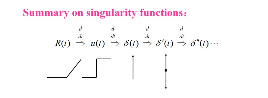
Signal Decomposition
$$ f(t) = f_D+f_A(t)\\ f(t)=f_e(t)+f_o(t)\\ f(t)=f_r(t)+jf_i(t)\\ f_r(t)=\frac{1}{2}\left[f(t)+f^*(t)\right]\\ f_i(t)=\frac{1}{2}\left[f(t)-f^*(t)\right] $$Pulse Component
$$ f(t)=\int_{-\infty}^{\infty}f(t_1)\delta(t-t_1)\mathrm dt_1 $$We also have orthogonal function decomposition(Chap.3, Chap.6).
System modeling and Classification
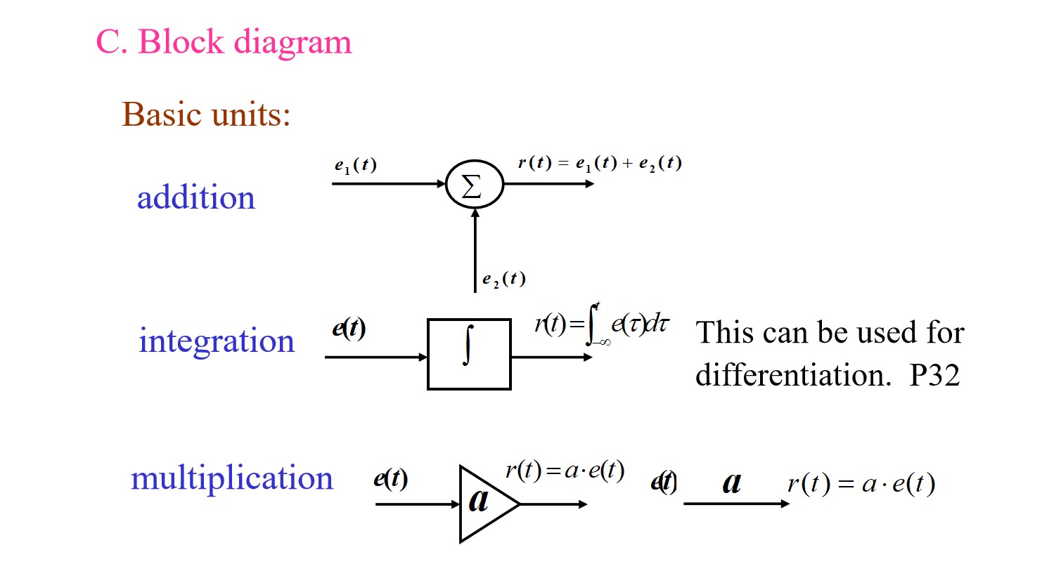
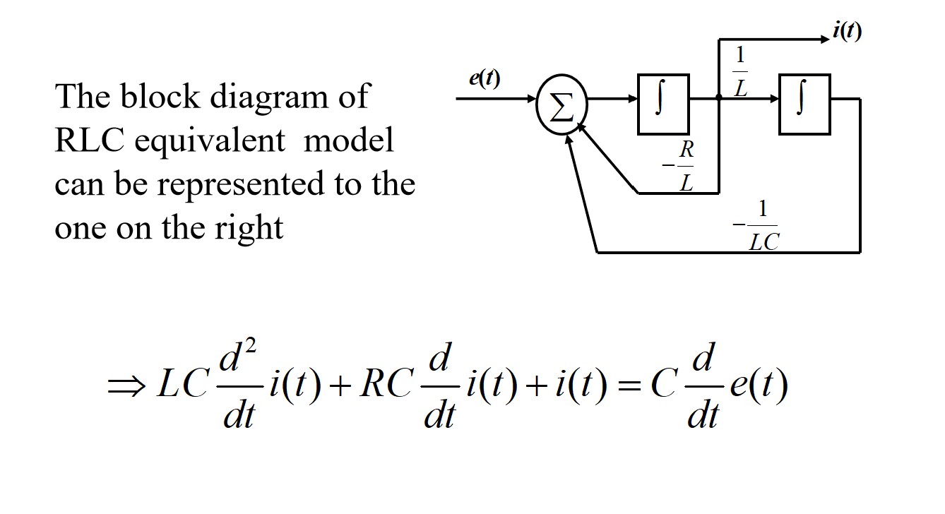
System model can be represented by math equation(including input-output description and state variables or state equation) graphic symbol and block diagrams.
We use the input-output description mostly. If controling something internal is needed, state euqtion is useful.
Block diagram:
System classification
Linear or Non-linear
$$ e_1(t)\rightarrow r_1(t), e_2(t)\rightarrow r_2(t)\Rightarrow\\ a_1e_1(t)+a_2e_2(t)\rightarrow a_1r_1(t)+a_2r_2(t) $$Time-variant or Time-invariant
Memory or Memoryless
with memory: dynamic system, differential equation
without memory: instant system, algebraic equation
Continuous or Discrete
Continuous Differential equation
Discrete Difference equation
Lumped- or Distributed-Parameter
Lumped: constant coefficient differential equation
Distributed: partial equation
Causal or Non-Causal
when $t<0, e(t)=0 \Rightarrow t<0, r(t)=0$ Generic definition?
the future state cannot have effect on now state. The state of causal system can only be determined by now and past states.
Reversible or irreversible
different input to different output, otherwise irreversible.
LTI System
Linearity
Linearity leads to superposition and homogeneity.
Time-Invariant
a time shift in the input results in a same time shift in the output.
$$ e(t)\rightarrow r(t)\Rightarrow e(t-t_0)\rightarrow r(t-t_0)\\ \lim_{\Delta t\rightarrow 0}\frac{e(t)-e(t-\Delta t)}{\Delta t}\rightarrow \lim_{\Delta t\rightarrow 0}\frac{r(t)-r(t-\Delta t)}{\Delta t}\\ \frac{\mathrm de(t)}{dt}\rightarrow \frac{\mathrm dr(t)}{dt} $$If every coefficient is time independent, the system is time invariant.
Time-Domain(TD) Analysis
$$ C_0\frac{d^nr(t)}{dt^n}+C_1\frac{d^{n-1}r(t)}{dt^{n-1}} + ... + C_nr(t)\\ =E_0\frac{d^me(t)}{dt^m}+E_1\frac{d^{m-1}e(t)}{dt^{m-1}}+...+E_me(t) $$Three Steps
- Homogeneous
- Particular
- Calculation on coefficients
Determining Coefficients
If functions are continuous, we can get their boundary conditions by determining the derivatives.
Then the coefficients can be solved by multipling the inverse of Vandermonde matrix with the boundary condition matrix.
Zero-input and -state Responses
Zero-input response The response caused by the initial state (i.e., energy originally stored in the system), and it is denoted by $r_{zi}(t)$
Zero-state response $r(0_-)\equiv 0$ , the response caused only by the external excitation and it is denoted by $r_{zs}(t)$

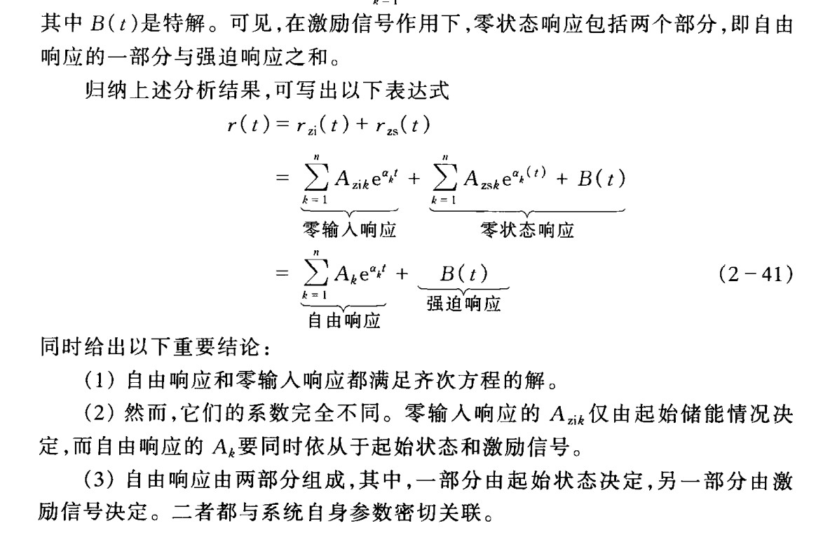
The combination of zero-input response and the zero-state response is not necessarily linear, since the existence of constant. If one of them vanishes, the other is linear.
Impulse and Step Responses
Impulse Response the zero-state response $h(t)$ to $\delta (t)$ , which can be equalized to the initial condition.
Note: normally $n>m$ .
Unit Step Response The zero-state response $g(t)$ to $u(t)$
There might be a forced term in $g(t)$ .
$$ g(t) = \int_0^th(\tau)d\tau $$Convolution
Zero-state required
$$ e(t) = \int_{-\infty}^{\infty}e(\tau)\delta(t-\tau)\mathrm d\tau\\ \Rightarrow r(t)=\int_{-\infty}^{\infty}e(\tau)h(t-\tau)\mathrm d\tau\\ \Rightarrow r(t)=e(t)*h(t) $$the definition of convoluiton:
$$ f_1(t)*f_2(t)=\int_{-\infty}^{\infty}f_1(\tau)f_2(t-\tau)\mathrm d\tau $$Integral interval $e(t)=0, \forall t<0$ , $h(t)=0,\forall t<0$ , so $r(t)=\int_0^t{e(\tau)h(t-\tau)\mathrm d\tau}$
The condition for applying convolution:
- For linear system ONLY
- For time variant systems, $h(t, \tau)$ means response at time $t$ generated by the impulse at time $\tau$ , then $r(t)=\int_0^th(t,\tau)e(\tau)\mathrm d \tau$ ; for time-invariant system is a special case, $h(t,\tau)=h(t-\tau)$ .
The Properties of Convolution The commutative property, the distributive property, the associative property
Differential:
$$ (f_1(t)*f_2(t))^\prime=f_1^\prime(t)*f_2(t) $$Integral
$$ \int f_1(t)*f_2(t)=f_1(t) * \int f_2(t) $$ $$ (f_1(t) * f_2(t))^{(i)}=f_1^{(j)}(t) * f_2^{(i-j)}(t) $$Convolution with $\delta (t)$ or $u(t)$
(1) $f(t) * \delta(t) = f(t)$
(2) $f(t) * \delta(t - t_0) = f(t-t_0)$
(3) $f(t) * u(t) = \int_{\infty}^{t}f(\tau)\mathrm d\tau$
(4) $f(t) * \delta^\prime(t) = f^\prime(t)$
Fourier Transform
Fourier Series
requirements:
- has finite number of discontinuities
- has finite number of maxima and minima
- $\int_{t_0}^{t_0+T_1} |f(t)|\mathrm dt < \infty$
note When $b_n=0$ , $\varphi_n = a_n > 0\ ?\ 0:\pi$
In the last part, the negative frequency is introduced for the convenience of the signal analysis. Therefore the amplitude is reduced to half.
FS for special functions
- Even function $c_n=a_n, \varphi_n = 0, F_n=F_{-n}=\frac 12 a_n$
- Odd function $a_0=0, a_n=0, \varphi_n=-\frac{\pi}{2}, F_n=F_{-n}=-\frac{1}{2}jb_n$
- Half-wave Odd (odd harmonic) function, $f(t)=-f\left(t\pm \frac{T_1}2{}\right)$ , contains only odd harmonics(both sine and cosine)
- Finite term series
FS for typical periodic signals
Periodic square wave
$$ f(t)=\frac{E\tau}{T_1}+\sum_{n=1}^{\infty}\frac{2E\tau}{T_1}\text{Sa}(\frac{n\omega_1\tau}{2}) $$- Spectrum is discrete with frequency spacing $\omega_1 = \frac{2\pi}{T_1}$ . When $T_1 \rightarrow \infty$ , the spectrum will be continuous.
- Amplitude: $\text{Sa}\left(\frac{n\pi\tau}{T_1}\right)$ or $\text{Sa} \left(\frac{n\omega_1\tau}{2}\right)$ , cross zero when $\omega_1 = \frac{2m\pi}{\tau}$
- Non-zero FS coefficients of a aperiodic signal are infinite with most energy concentrated at low frequency components (within $\left(-\frac{2\pi}{\tau},\frac{2\pi}{\tau}\right)$ ). Thus we define the bandwith $B_{\omega} = \frac{2\pi}{\tau}$
Periodic symmetric square wave
Since the spectrum crosses zero when $\omega_1 = \frac{2m\pi}{\tau}$ , the even harmonic vanishes. Also the sine component vanishes.
$$ c_n = \frac{2E\tau}{T_1}\left|\text{Sa}\left(\frac{n\omega_1\tau}{2}\right)\right|\\ f(t) = \frac{2E}{\pi}\left[\cos(\omega_1t) - \frac{1}3\cos(3\omega_1t) + \frac{1}{5}\cos(5\omega_1t)-...\right] $$Periodic Serrated Pulse
$$ f(t) = \sum_{n = 1}^\infty \frac{E}{n\pi}(-1)^{n+1}\sin (n\omega_1t) $$Periodic Triangular Pulse
$$ f(t)=\frac E2 + \frac{4E}{\pi^2}\sum_{n=1}^\infty\frac{1}{n^2}\sin^2\left(\frac{n\pi}{2}\right)\cos(n\omega_1t)\\=\frac E2 + \frac{4E}{\pi^2}\sum_{n=1}^\infty\frac{1}{(2n-1)^2}\cos((2n-1)\omega_1t) $$consine of non-negative values
$$ f(t) = \frac E\pi - \frac{2E}{\pi}\sum_{n=1}^\infty\frac{1}{n^2-1}\cos(\frac {n\pi}2)\cos(n\omega_1t) $$cosine of absoulute values
$$ f(t) = \frac{2E}{\pi} + \frac{4E}{\pi}\sum_{n=1}^\infty (-1)^{n+1}\frac{1}{4n^2-1}\cos(2n\omega_0t) $$其中 $\omega_0$ = $2\omega_1$
Fourier Transform
The case where $T_1\rightarrow \infty$ . Signal becomes aperiodic.
Also, $\omega_1\rightarrow 0$ results in the continuous frequency axis. For square wave the magnitude $\frac{E\tau}{T_1}\rightarrow 0$ .
$$ f(t) =\sum_{n=-\infty}^{\infty}F(n\omega_1)e^{jn\omega_1 t}\\ F(n\omega_1) = \frac 1T_1\int_{-\frac {T_1}2}^{\frac {T_1}2}f(t)e^{-jn\omega_1t}\mathrm dt $$We use spectrum density to replace spectrum, making the magnitude dropping to zero remain its meaning.
$$ \frac{F(n\omega_1)}{\omega_1} = \frac{1}{2\pi}\int_{-\frac {T_1}2}^{\frac {T_1}2}f(t)e^{-jn\omega_1t}\mathrm dt\\ F(\omega) = \lim_{\omega_1\rightarrow 0}\frac{2\pi F(n\omega_1)}{\omega_1}=\lim_{T_1\rightarrow \infty}\int_{-\frac {T_1}2}^{\frac {T_1}2}f(t)e^{-jn\omega_1t}\mathrm d t=\int_{-\infty}^\infty f(t)e^{-j\omega t}\mathrm d t\\ f(t) = \sum_{n=-\infty}^{\infty}F(n\omega_1)\cdot \frac{1}{\omega_1}e^{jn\omega_1 t} \Delta(n\omega_1) = \frac{1}{2\pi}\int_{-\infty}^\infty F(\omega)e^{j\omega t}\mathrm d\omega $$ $$ F(\omega) = |F(\omega)|e^{j\varphi(\omega)} $$The fourier transfrom is continuous waveform, where every frequency has no energy but energy density, used to analyse aperiodic function.
Sufficient condition, but not necessary.
$$ \int_{-\infty}^\infty |f(t)|\mathrm dt<\infty $$FT for typical aperiodic signals
Rectangular pulses
$$ F(\omega) = \int_{-\tau/2}^{\tau/2} Ee^{-j\omega t}\mathrm dt = E\tau \text{Sa}\left(\frac{\omega \tau}{2}\right) $$Raised Cosine Signal
$$ f(t) = \frac{E}{2}(1+\cos\frac{\pi t}{\tau})(u(t+\tau) - u(t - \tau))\\ F(\omega) = \int_{-\tau}^{\tau}(1+\cos\frac{\pi t}{\tau})\mathrm dt = \frac{E\tau}{1 - \left(\frac{\omega \tau}{\pi}\right)^2}\text{Sa}({\omega \tau}) $$More compacted than square signal( $|F(\omega)|\propto \frac 1{\omega^3}$ ). An explanation is that the raised cosine has no discontinuities.
Generally:
- $f(t)$ has discontinuities, $|F(\omega)|\propto \frac 1{\omega}$
- $\frac{d}{dt}f(t)$ has discontinuities, $|F(\omega)|\propto \frac 1{\omega^2}$
- $\frac{d^2}{dt^2}f(t)$ has discontinuities, $|F(\omega)|\propto \frac 1{\omega^3}$
The width $\tau$ of the raised cosine signal is defined at $\frac E2$ rather than at the bottom, making it easy to compare with
the rectangular pulse of same width. The first zeros of the
frequency spectrum are identical.
raised consine is energy-concentrative and has been widely used in digital communications.
Single-sided exponential singal
$$ f(t) = e^{-at}u(t)\\ F(\omega) = \frac{1}{a+j\omega} $$Two-sided, anti-symmetric exponential signal
$$ f(t) = -e^{at}u(-t) + e^{-at}u(t)\\ F(\omega) = \frac{-2j\omega}{a^2+\omega^2} $$Sign function
$$ \text{sgn}(t) = u(t) - u(-t)\\ F(\omega) = \lim_{a\rightarrow 0}\frac{-2j\omega}{a^2+\omega^2}= \frac{2}{j\omega} $$Gaussian singal
$$ f(t) = Ee^{-\left(\frac{t}{\tau}\right)^2}\\ F(\omega) = \sqrt \pi E\tau e^{-\left(\frac{\omega\tau}{2}\right)^2} $$Sinc Function
$$ f(t) = \frac{E}{\pi}\frac{\sin(\omega_c t)}{t}\\ F(\omega) = E(u(\omega - \omega_c ) + u(\omega + \omega_c ))\\ $$FT on impulse and step functions
$$ \mathcal F[\delta(t)] = 1\\ \mathcal F[1] = 2\pi \delta(\omega) $$The spectrum of impulse function covers the entire frequency range. The interferences caused by a variety of electric sparks always cover the full frequency range.
$$ \mathcal F[\delta^\prime (t)]= j\omega\\ \mathcal F[\delta^{(n)}(t)] = (j\omega)^n $$ $$ \mathcal F[u(t)] = \pi \delta(\omega) + \frac{1}{j\omega} $$Due to the DC component in u(t), an impulse exists.
Properties of FT
Symmetry $\mathcal F[F(t)]= 2\pi f(-\omega)$ , if $f(t)$ is a even function, $\mathcal F[F(t)]= 2\pi f(\omega)$
Linearity $\mathcal{F}[\Sigma_{i=1}^{n}a_if_i(t)] = \Sigma_{i=1}^{n}a_iF_i(\omega)$
Odd-Even, Imaginary-Real $f(t) = f_e(t)+f_o(t)$ , then
$$ \begin{align*} F(\omega) &= \int_{-\infty}^\infty f(t)\cos \omega t \mathrm dt -j\int_{-\infty}^\infty f(t)\sin \omega t \mathrm dt\\ &=R(\omega)+jX(\omega)\\ &=\int_{-\infty}^\infty f_e(t)\cos \omega t \mathrm dt -j\int_{-\infty}^\infty f_o(t)\sin \omega t \mathrm dt\\ \end{align*}. $$ $R(\omega)$ is an even function of $\omega$ , $X(\omega)$ is an odd function of $\omega$ . $|F(\omega) = \sqrt{R^2(\omega)+F^2(\omega)}|$ is even function. $\varphi(\omega) = \tg^{-1}\frac{R(\omega)}{X(\omega)}$if $f(t)$ is real and even, then $f(t)=f_e(t), F(\omega)=R(\omega)$ , the phase shift is $0$ or $\pi$ .
if $f(t)$ is real and odd, $f(t) = f_o(t)$ , then $F(\omega)=jX(\omega)$ , $F(\omega)$ has only imaginary part and is odd, the phase shift is $\pm \frac{\pi}{2}$
Scaling $\mathcal{F}[f(at)]=\frac 1{|a|}F\left(\frac{\omega}a\right)$ Expansion in TD results in Compression in FD.
Time Shifting $\mathcal{F}[f(t\pm t_0)] = F(\omega)e^{\pm j\omega t_0}$
Frequency Shifting $\mathcal F[f(t)e^{\pm j\omega_0t}] = F(\omega\mp\omega_0)$
Differentiation property $\mathcal F\left[\frac{\mathrm d}{\mathrm dt}f(t)\right] = j\omega F(\omega)$
$\mathcal F\left[\frac{\mathrm d^n}{\mathrm dt^n}f(t)\right] = (j\omega)^n F(\omega)$ $\mathcal F\left[\frac{\mathrm d^n}{\mathrm d\omega^n}F(\omega)\right] = (-jt)^nf(t)$Integration Property $\mathcal{F}\left[\int_{-\infty}^t f(\tau)\mathrm{d} \tau\right] = \frac{F(\omega)}{j\omega} + \pi F(0)\delta(\omega)$
Convolution theorem
$$ \mathcal F[f_1(t)* f_2(t)] = F_1(\omega)F_2(\omega)\\ \mathcal F[f_1(t)\cdot f_2(t)] = \frac 1{2\pi} F_1(\omega) * F_2(\omega) $$FT for Periodic Signals
$$ \mathcal F[\cos (\omega_0 t)] = \pi [\delta(\omega + \omega_0) + \delta(\omega - \omega_0)]\\ \mathcal{F} [\sin (\omega_0 t)] = j\pi [\delta(\omega+\omega_0) + \delta(\omega - \omega_0)] $$FT for periodic of $T_1$ & $\omega_1=2\pi/T_1$
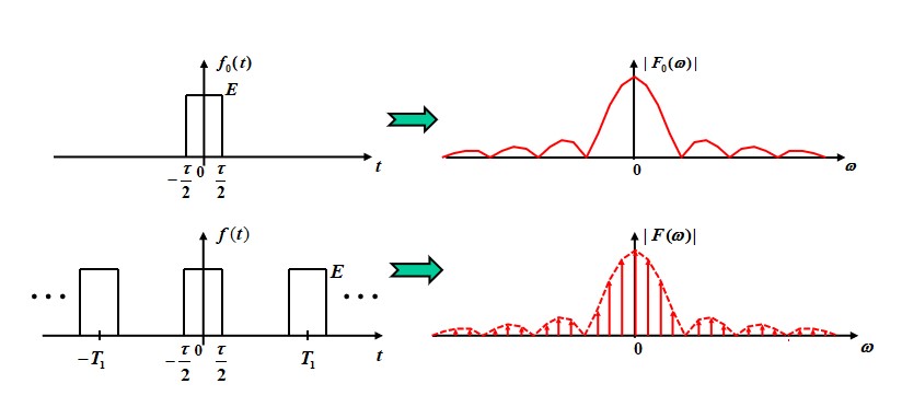
$$ \mathcal F[f(t)] = 2\pi\sum_{n=-\infty}^{+\infty} F_n\delta(\omega - n\omega_1)\\ F_n = \frac 1{T_1}\int_{-T_1/2}^{T_1/2}f(t)e^{-jn\omega_1 t}\mathrm dt = \frac{1}{T_1}F_0(\omega)\vert_{\omega =n\omega_1} $$Where $F_0(\omega)$ is the FT considering waveform of $f(t)$ only in $|t|\le T_1/2$ .
example:
$$ f(t) = \sum_{n=0}^{\infty}\delta(t-nT_1), F_n=\frac{1}{T_1}\\ F(\omega) = \frac{2\pi}{T_1}\sum_{n=0}^{\infty}\delta(\omega - n\omega_1)=\omega_1\sum_{n=0}^{\infty}\delta(\omega - n\omega_1) $$ $$ F_0(ω) \text{ determines the profile of } F(ω)\\ T_1\text{ determines the density of the impulses }\\ T_1↑, ω_1↓\text{, intensity of harmonics}↓\\ T_1↓,ω_1↑\text{, intensity of harmonics}↑\\ $$
In the same way:
FT for periodically sampled signals
$$ F(\omega) = \mathcal F[f(t)]\\ P(\omega) = \mathcal F[p(t)]\\ f_s(t) = f(t)p(t)\\ F_s(\omega) =\frac{1}{2\pi} F(\omega) * P(\omega) $$Then,
$$ P(\omega) = 2\pi \sum_{n = -\infty}^{+\infty} P_n\delta(\omega - \omega_s)\\ F(\omega) * P(\omega) = 2\pi \sum_{n = -\infty}^{+\infty} P_nF(\omega - n\omega_s)\\ F_s(\omega) = \sum_{n = -\infty}^{+\infty} P_nF(\omega - n\omega_s) $$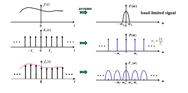
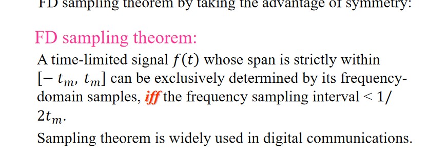
For the frequency-domain sampling:
$$ F_1(\omega) = F(\omega)P(\omega)\\ P(\omega) = \sum_{n=-\infty}^{+\infty} \delta(\omega - n\omega_1)\\ f_1(t) = f(t) * \frac{1}{\omega_1}\sum_{n=-\infty}^{+\infty} \delta(t - nT_1) = \frac{1}{\omega_1}\sum_{n=-\infty}^{\infty} f(t-nT_1) $$The Sampling Theorem
$$ \omega_s \ge 2\omega_m $$A band-limited signal whose spectrum is strictly within $[0, f_m]$ could be uniquely determined by the samples on itself, if and only if the sampling interval $T_s \le 1/(2f_m)$ .
$T_s = \frac{1}{2f_m}$ is called the **Nyquist interval**. $2f_m$ is called the **Nyquist frequency**.对于单频信号,奈奎斯特频率的采样可能会出现问题。例如正弦信号,每次采样都采在零点上,那就没法复现信号。单频信号没法描述带宽。
A FD verison:
L Transform
Unilateral L-transform
$$ F(s) = \int^{\infty}_{0}f(t)e^{-st}\mathrm dt, s=\sigma+j\omega\\ f(t)=\frac{1}{2\pi j}\int_{\sigma-j\infty}^{\sigma+j\infty}F(s)e^{st}\mathrm ds $$ $F(s) = \mathcal{L}[f(t)]$ is called image function, $f(t) = \mathcal{L}^{-1}[F(s)]$ is called primitive function.assuming that $f(t)$ is causal and always 0 if $t<0$ .
$$ \mathcal L \left[\frac{\mathrm df(t)}{\mathrm dt}\right] = -f(0) + sF(s) $$The initial state is automatically included in differential equation.
We define the unilateral L-Transform as:
$$ F(s) = \int_{0_-}^{\infty}f(t)e^{-st}\mathrm dt\\ \mathcal L \left[\frac{\mathrm df(t)}{\mathrm dt}\right] = -f(0_-) + sF(s) $$Conditions for L-Transform:
- Limited discontinuities
- Exponential order
The strong attenuation factor can make the function convergent.
Region of Convergence (ROC)
Axis of convergence
Coordinate of convergence $\sigma_0$
Comman LT Pairs
$$ \begin{align*} f(t)&\Rightarrow F(s)\\ \delta(t) &\Rightarrow 1\\ u(t) &\Rightarrow \frac 1s\\ e^{-at} &\Rightarrow \frac{1}{s+a}\\ t^n & \Rightarrow \frac{n!}{s^{n+1}}\\ \sin (\omega t)&\Rightarrow \frac{\omega}{s^2 + \omega^2}\\ \cos (\omega t)&\Rightarrow \frac{s}{s^2+\omega^2}\\ \end{align*} $$Properties of LT
Linarity
$$ \mathcal L [k_1f_1(t) + k_2f_2(t)] = k_1F_1(s) + k_2F_2(s)\\ $$Differentiation
$$ \mathcal L \left[\frac{\mathrm d f(t)}{\mathrm d t}\right] = sF(s) - f(0_-) $$Intergration
$$ \mathcal L\left[\int_{-\infty}^t f(\tau)\mathcal d\tau\right]=\frac{F(s)}{s} + \frac{f^{(-1)}(0)}{s} $$Time Shifting
$$ \mathcal L\left[f(t-t_0)u(t-t_0)\right] = e^{-st_0}F(s) $$Use $u(t-t_0)$ to avoid nagative part of $f(t)$ emerges.
Frequency Shifting
$$ \mathcal L[f(t)e^{-at}] = F(s+a) $$Scaling
$$ \mathcal L[f(at)] = \frac 1a F\left(\frac{s}{a}\right) $$s-Domain Differentiation
$$ \frac{\mathrm d}{\mathrm ds}\mathcal L[f(t)] = \mathcal L[-tf(t)] $$s-Domain Differentiation
$$ \int_s^\infty F(s) = \mathcal{L}\left[\frac{f(t)}{t}\right] $$Initial value
$$ f(0_+) = \lim_{s\rightarrow\infty}sF(s) $$Final value
$$ \lim_{t\rightarrow\infty} f(t) = \lim_{s\rightarrow0} sF(s) $$Generalized limit: $\lim_{t\rightarrow\infty} \sin(\omega t)=0$
Convolution
$$ \mathcal L[f_1(t)*f_2(t)] = F_1(s)F_2(s) $$Applications
Differential Equations
$$ F(s) = \frac{A(s)}{B(s)} = \frac{a_ns^n + a_{n-1}s^{n-1} + \cdots + a_1s + a_0}{b_ms^m + b_{m-1}s^{m-1} + \cdots + b_1s + b_0} % The division of two polynomials $$(assume that $n<m$ )
The roots of numerator is called zeros, while the roots of denominator is called poles.
Unknown function F(s) can be represented by the ratio of two polynomials if all initial states are 0.
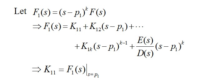
- real poles
- complex conjugate poles
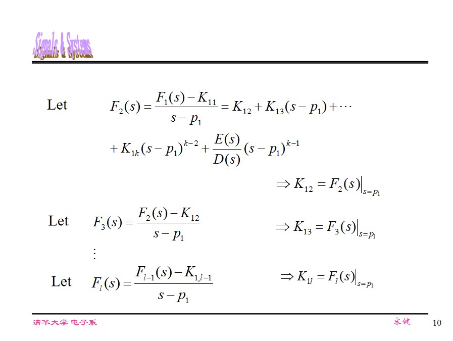
- Multiple poles
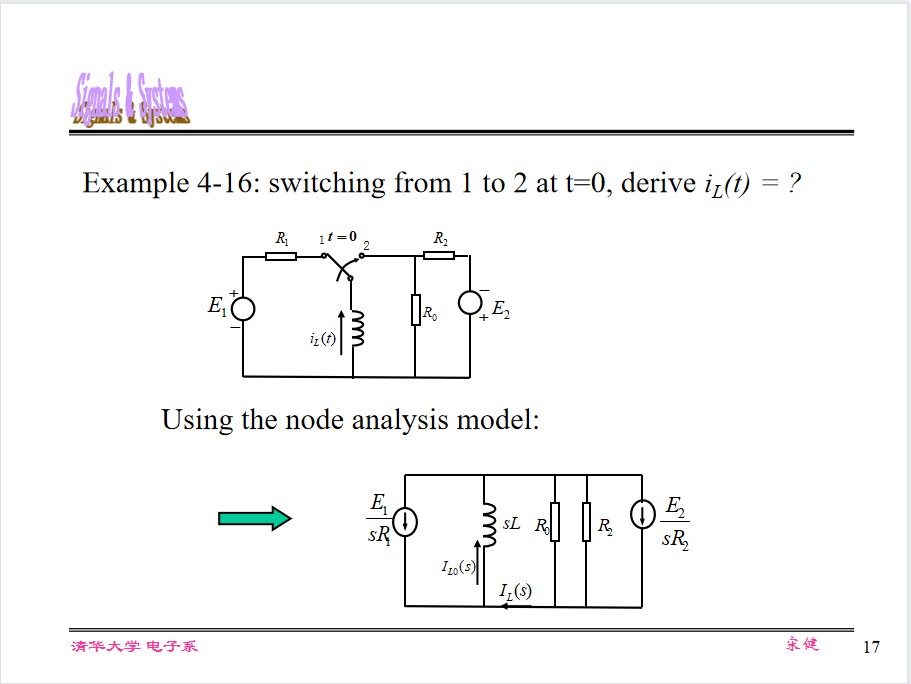
Circuit model:
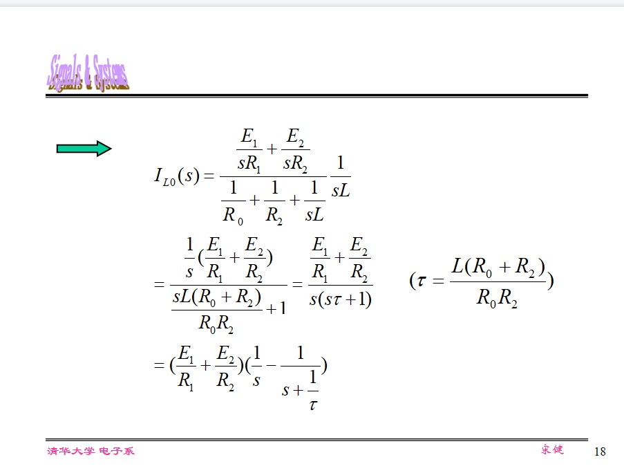
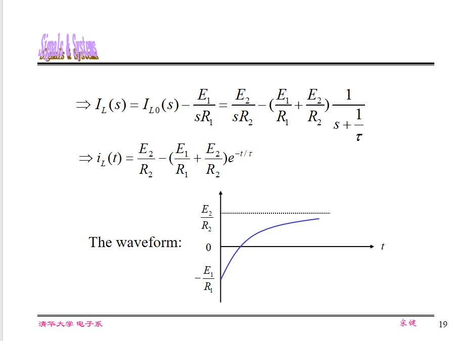
Use initial value and final value to verify it.
System Function
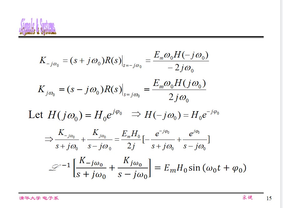
$$ \begin{cases} R(s) = H(s) \cdot E(s)\\ r(t) = h(t) * e(t) \end{cases} \Rightarrow H(s) = L[h(t)] $$Driving point function & transfer function
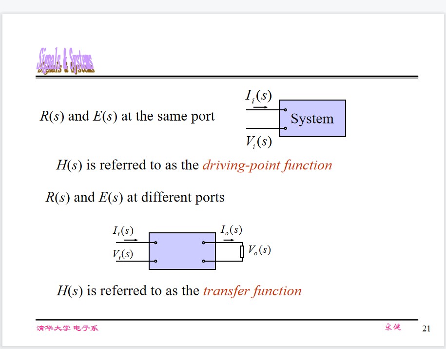
L-transform can be used in the following analysis:
- TD characteristics (response decomposition)
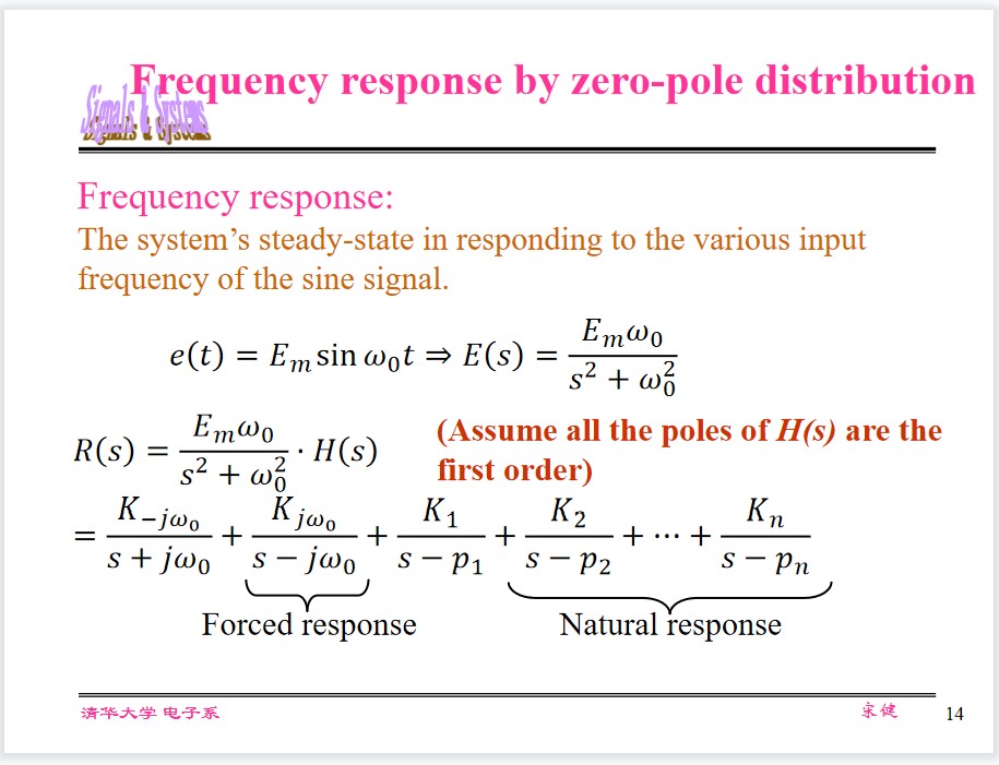
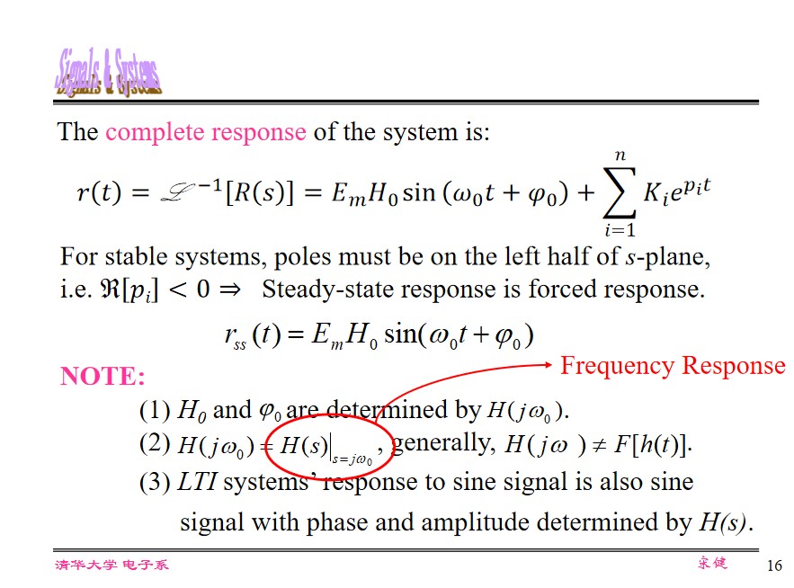
- FD characteristics (steady-state with sine signal input,applications such as filtering)
- Stability (active network, feedback, oscillator, control system)
TD characteristics by 0-point distribution
Three cases:
- Real poles
- Complex conjugate poles
- Real pole of high-order
- Zero pole of H(s)
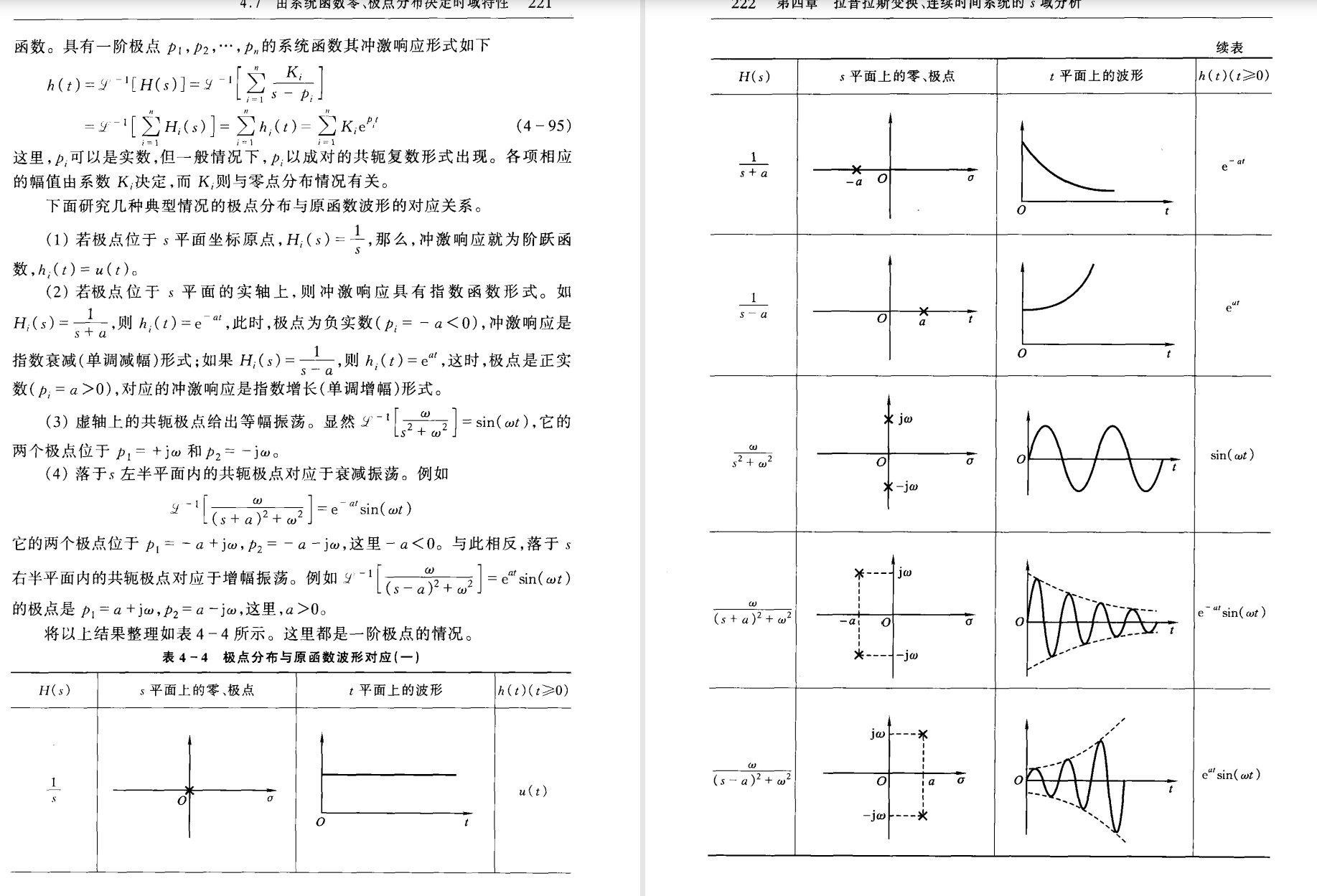
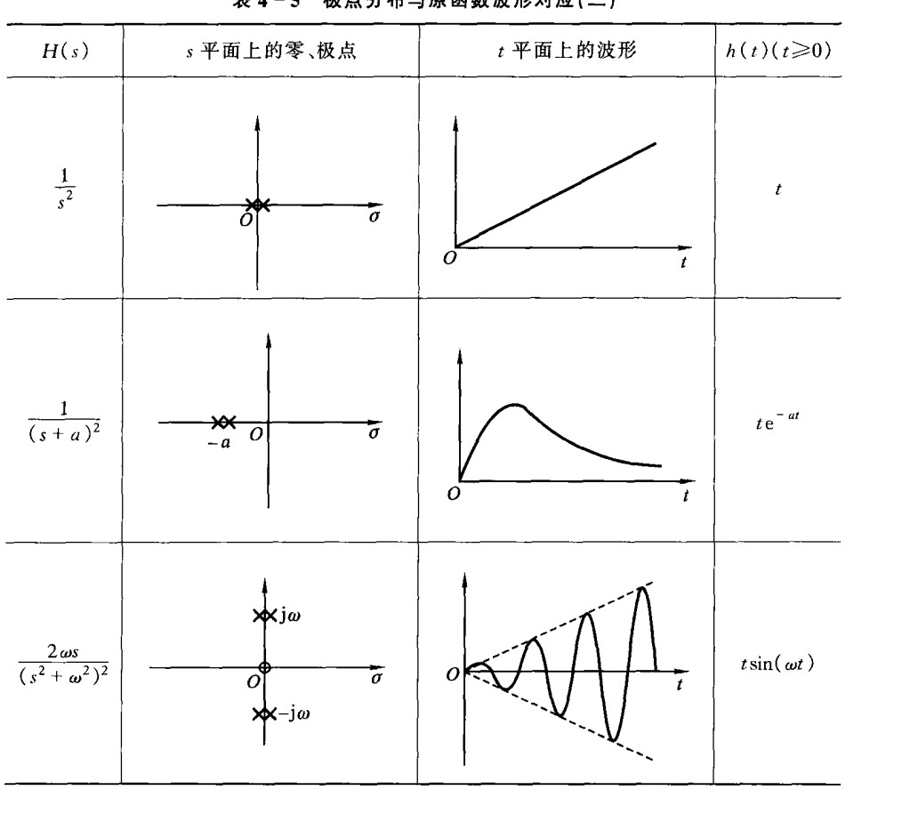
Zero only affects the phase and amplitude, while the shape and type of waveform is determined by the poles.
- pole distribution $\Leftrightarrow$ corresponding natural/forced responses
The natural response of $r(t)$ is only related to $p_{hk}$ , while the forced response is only related to $p_{ek}$ .
$K_{hk}$ , $K_{ek}$ are related to both $H(s)$ and $E(s)$ .However natural and forced responses could not be completely separated, if there exists $k, k^\prime$ satisfying $p_{hk}=p_{ek^\prime}$ .
$p_{hi}$ are called natural frequency of the system.However, some common factors may be eliminated:
$$ \frac{(s+1)}{(s+1)(s+2)} = \frac{1}{(s+2)} $$ $$ H(s) = \frac{\Delta_{jk}}{\Delta} $$All the poles of $H(s)$ are the natural frequencies of the system, but $h(t)$ may not include all the natural frequencies(but the root of $\Delta$ contains all natural frequencies).
In most cases:
$$ \text{Re}(p_{hi}) < 0, \text{Re}(p_{ei}) = 0 $$Thus the natural response is transient, while the forced response is steady-state.
However, some natural response can be steady-state(conjugate poles of $Re(p_{hi})$ ), while some forced response can be transient.
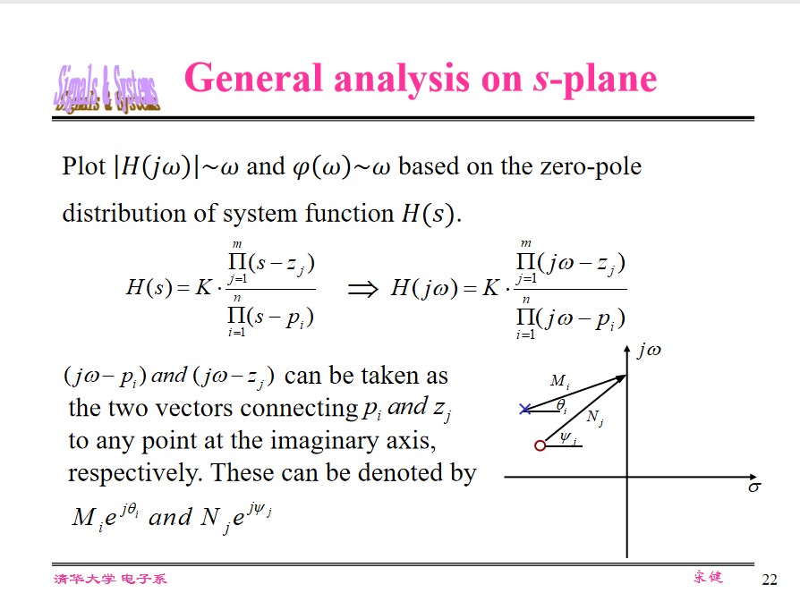
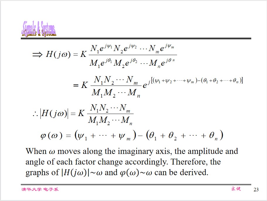
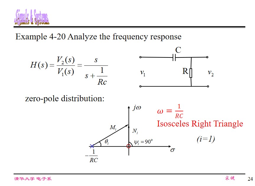
for band-pass filter,
BW is where Peak(dB) - 3dB
for low-pass filter,
BW = $f_{\text{cut-off}}$
According to the sampling theorem, the signal bandwith is often determined by the first zero of the spectrum.
All Pass Systems
$$ R_e(p_i) = -R_e(z_i)\\ I_m(p_i) = I_m(z_i) $$The Amplitude is const., while the phase can change.
Minimum-phase system/function
Definition: A stable system with poles on left-half s-plane is called minimum-phase system/function, if all the zeros are also on left-half s-plane or at the jω-axis. Otherwise is a non-minimum-phase system/function.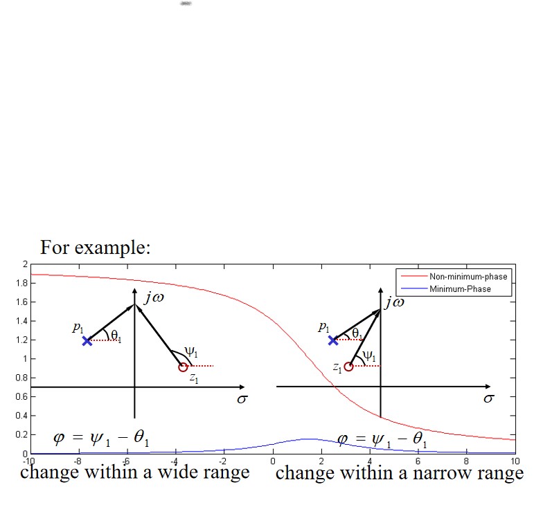
Property: A non-minimum-phase function can be represented as the product of a minimum-phase function and an all-pass function.
Stability of Linear System
A system is considered to be stable if bounded input always leads to bounded output.
Bounded-input, Bounded-output(BIBO)
The necessary & sufficient conditions for BIBO:
$$ \int_{-\infty}^\infty|h(t)|\mathrm dt \le M $$Poles are:
- on the left half-plane: $\lim_{t\rightarrow \infty}[h(t)] = 0$ , stable system
- on the right half-plane, or at $j\omega$ -axis with order of more than one: $\lim_{t\rightarrow \infty}[h(t)] = \infty$ , unstable system
- at $j\omega$ -axis with order of one: $h(t)$ is non-zero or oscillated with equal amplitude, critical stable system
Two-sided (Bilateral) LT
$$ F_B(s) = \int_{-\infty}^\infty f(t)e^{-st}\mathrm{d} t $$- t starts from −∞, i.e., non-causal signal as the input
or regarding the initial condition as the input. - Easily to be associated with F-transform and Z-
transforms
We determine the ROC by:
$$ \lim_{t\rightarrow \infty} f(t)e^{-\sigma t} = 0\\ \lim_{t\rightarrow -\infty} f(t)e^{-\sigma t} = 0 $$NOTE:
- If no overlap between the two constraints, then $F_B(s)$ does not exist.
- $F_B(s)$ and $f(t)$ are not uniquely corresponding to each other.( $\int_{-\infty}^\infty u(t)e^{-st}\mathrm{d} t = \frac{1}{s}$ , $\int_{-\infty}^\infty -u(-t)e^{-st}\mathrm{d} t=\frac{1}{s}$ )
- Two-sided L-Transform shares almost all the properties with its single-sided counterpart except for the initial-value theorem.
- Two-sided L-Transform has very limited applications as most continuous-time systems are causal.
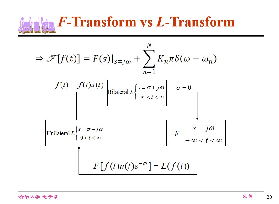
**Relationship between LT and FT **
- $\sigma_0 > 0$ , $F(\omega)$ does not exist
- $\sigma_0 = 0$ , impulse appears in $F(\omega)$
- $\sigma_0 < 0$ , $F(\omega)$ exists, $F(\omega) = F(s)|_{s=j\omega}$
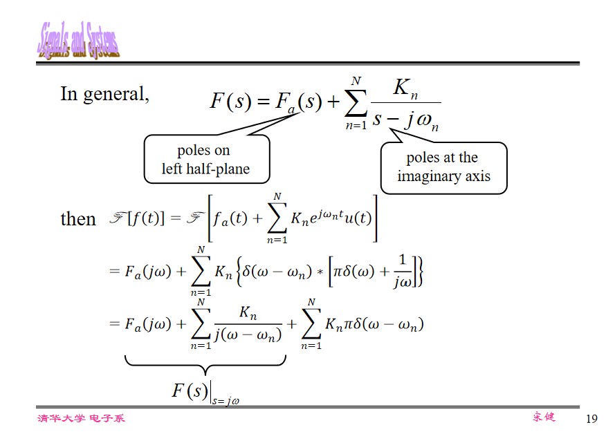
(The LT above is unilateral LT.)
Extra Attention
$1 + e^{-s}$ also has zero(many!). Note that if it is on the denominator.FT in Telecom. Systems
System discussed in this chapter are strictly stable:
$$ \mathcal{F}[f(t)] = F(s)|_{s=j\omega} $$Because even for critical stable system, FT is not the same as LT(containing $\delta$ ), there will be ambiguity between $H(j\omega)$ and $H(s)|_{s=j\omega}$ .
For every freq. component, it is reshaped in its phase and amplitude by the system function when passing through the system, related with its frequency. Thus the system can distort the original signal.
Distortion
2 types of distortion:
- Non-linear distortion (new frequency components)
- Linear distortion (without new frequency components), just the amplitude and/or phase distortion.
Distortionless transmission
$$ e(t)\rightarrow ke(t - t_0) $$ $$ R(j\omega) = \int_{-\infty}^\infty ke(t -t_0)e^{-j\omega t}\mathrm dt=ke^{-j\omega t_0}\int_{-\infty}^\infty e(x)e^{-j\omega x}\mathrm dx=ke^{-j\omega t_0} E(j\omega) $$So, $H(j\omega) = ke^{-j\omega t_0}$ , $h(t)=K\delta(t - t_0)$ .
The Amplitude is frequency independent, $BW\rightarrow \infty$ .
Phase response is linear at negative slope.
The impulse response of a distortionless linear system is
also an impulse.
The physical scenario: group delay.
$$ \tau = -\frac{\mathrm d\varphi (\omega)}{\mathrm d\omega} $$Condition for phase distortionless property: the group delay remains a constant.
Filter
Ideal Low pass (LP) Filter
$$ H(j\omega) = \begin{cases} 1 \cdot e^{-j\omega t_0}, &|\omega|< \omega_c,\\ 0, &|\omega|> \omega_c. \end{cases} $$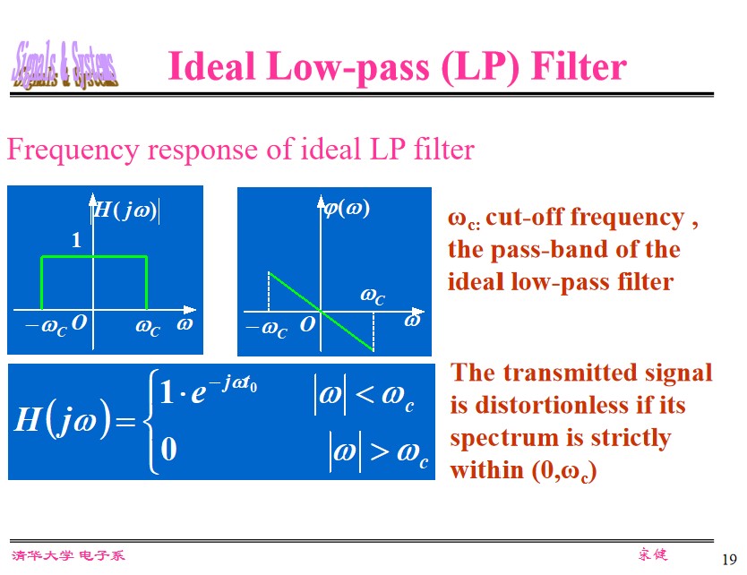
The Impulse response of Ideal LP
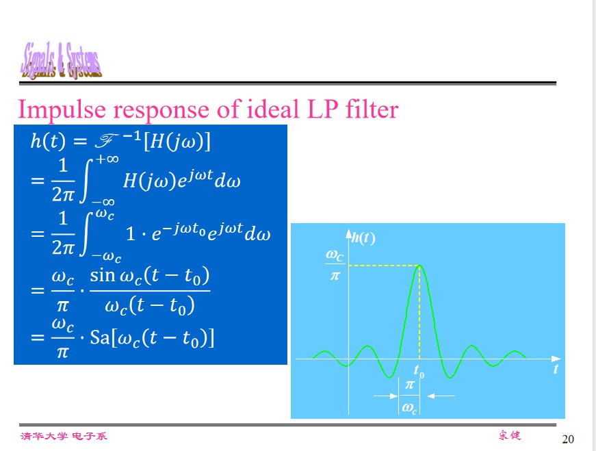
- Severe distortion. $BW_{\delta(t)}\rightarrow \infty$ , but $BW_{\text{Lowpass}}=\omega_c$ , the higier frequency is eliminated.
- Non-causal. When $t\lt 0$ , $h(t)\ne 0$ .
Unit-step response of Ideal LP
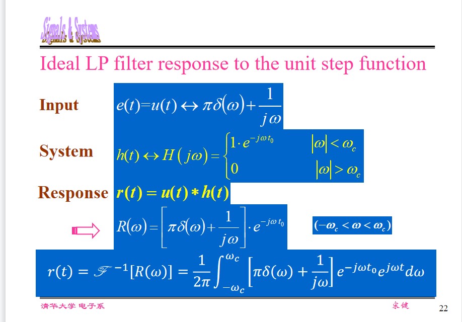
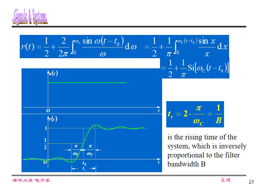
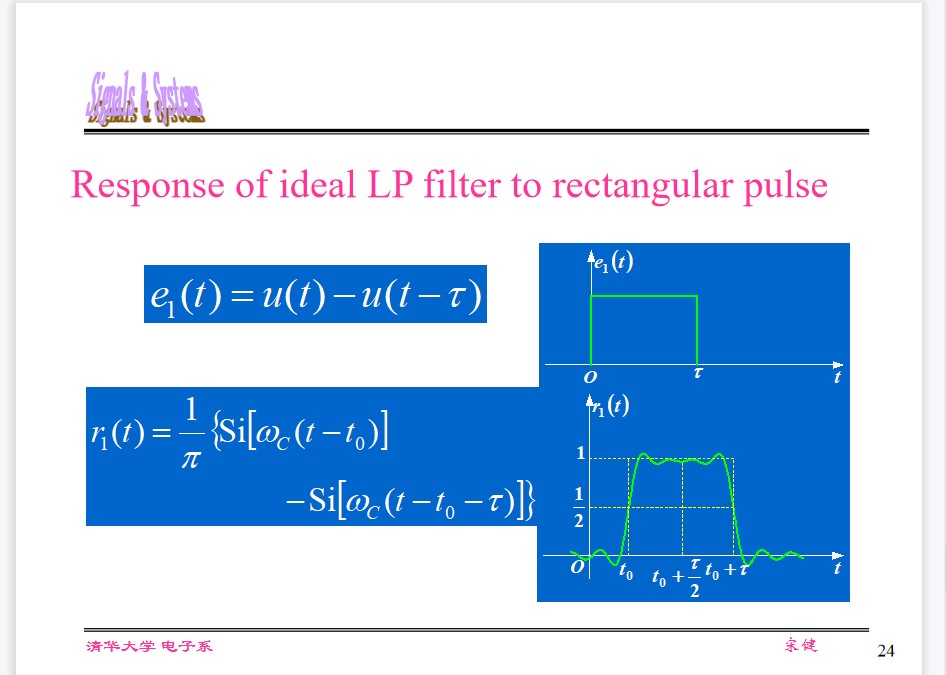
The response is similar to the input if $\frac{1}{2}=\frac{\pi}{\omega_c}\llless \tau$ .
Gibbs phenomenon: 9% overshoot at discontinuity. Use other window functions can eliminate this, e.g. raised-cosine window.
Modulation and demodulation
Means of modulation:
Spectrum shifting
$f(t) = g(t)\cos(\omega_0t)$ , $F(\omega) =\frac{1}{2\pi} G(\omega) * \pi[\delta(\omega - \omega_0) + \delta (\omega + \omega_0)] = \frac{1}{2}[G(\omega + \omega_0) + G(\omega - \omega_0)]$ .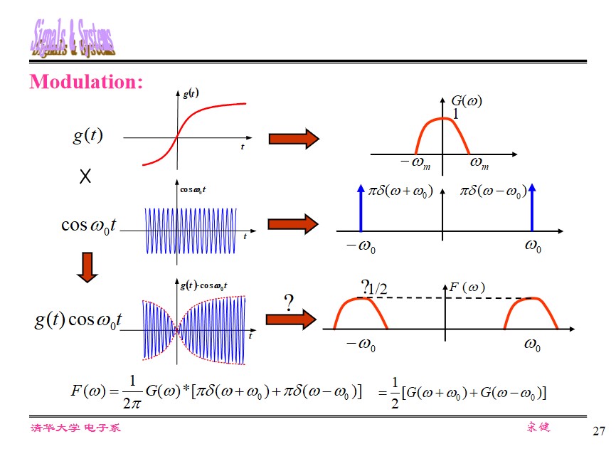
Demodulation:
coherent demodulation
$g_0(t)=[g(t)\cos(\omega_0 t)]\cos(\omega_0t) = \frac{1}{2}g(t) + \frac{1}{2}g(t)\cos2\omega_0t$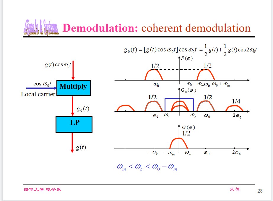
Envelope Detection
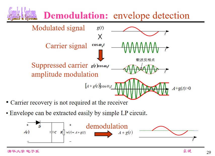
Applications of BPF
Window Function
(Page 304)
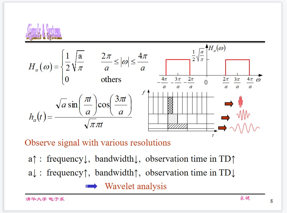
Recover Continuous Time signal from its Samples
Analysis on signal after band-pass filter
Page 301
Sampling with impulse func.
FD analysis:
Sampled signal(By impulse function):
$$ F_s(\omega) = \frac{1}{T_s}\sum_{n=-\infty}^\infty F(\omega - n\omega_s) $$Ideal LP Filter:
$$ H(j\omega) = \begin{cases} T_s, &|\omega|< \omega_c,\\ 0, &|\omega|> \omega_c. \end{cases} $$Recovered signal:
$$ F(\omega) = F_s(\omega) \cdot H(\omega) $$TD analysis:
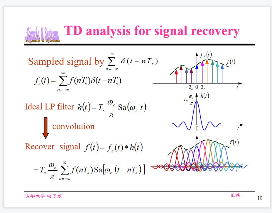
Sampled signal:
$$ f_s(t) = \sum_{n=-\infty}^\infty f(nT_s)\delta(t - nT_s) $$Ideal LP Filter:
$$ h(t) = T_s\frac{\omega_c}\pi \text{Sa}(\omega_c t) $$Recovered signal:
$$ f(t) = f_s(t) * h(t) = T_s\frac{\omega_c}\pi \sum_{n=-\infty}^\infty f(nT_s) \text{Sa}(\omega_c (t-nT_s)) $$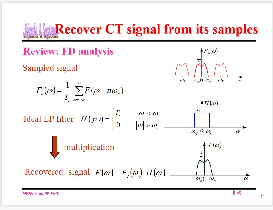
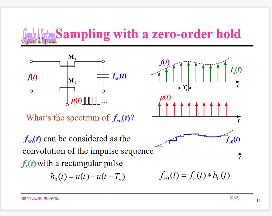
Sampling with a zero-order hold
LP Filter for compensation
$$ H_{0r}(\omega) = \begin{cases} \frac{1}{\text{Sa}(\frac{\omega T_s}{2})}e^{j\omega T_s/2}, &|\omega| \le \omega_s/2,\\ 0, &|\omega|> \omega_s/2. \end{cases} $$Linear phase response is OK! No needed for delay compensation.
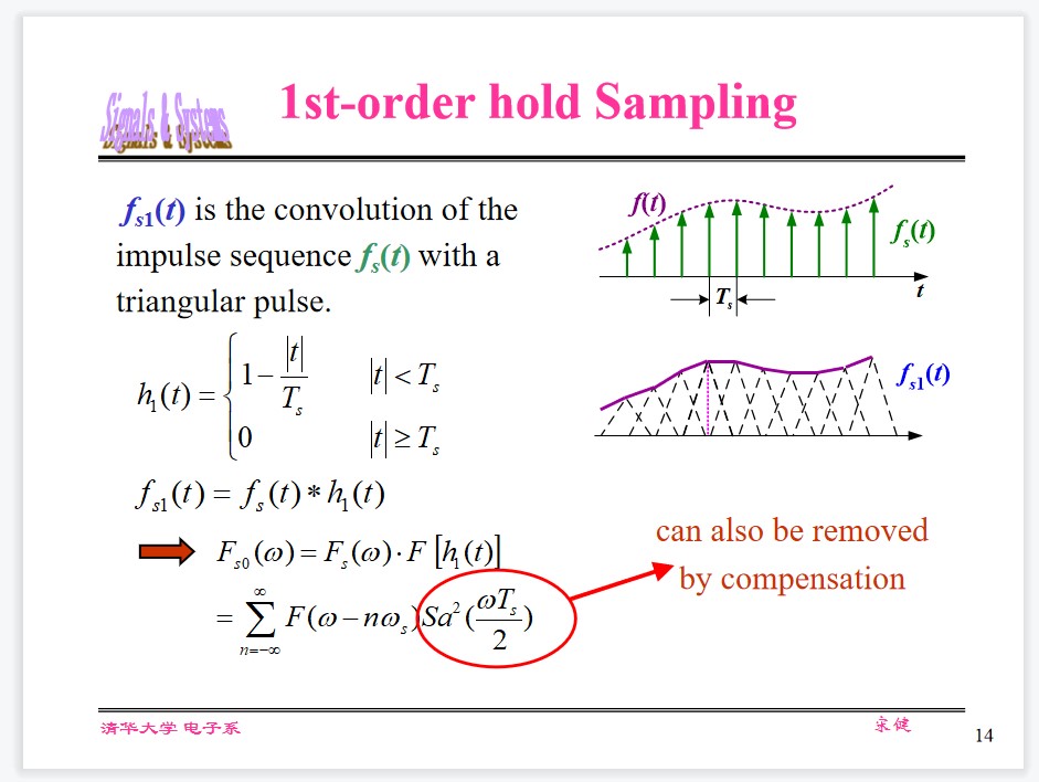
1st-order hold Sampling
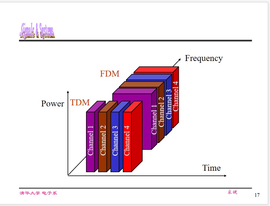
Mulitplexing FDM and TDM
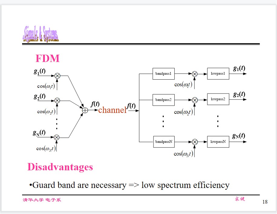
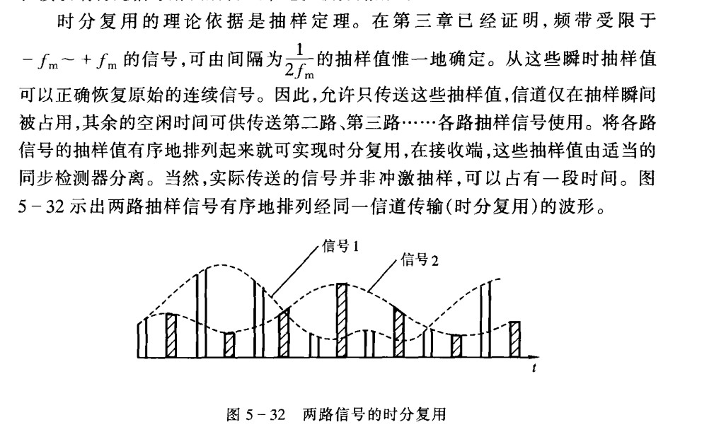
Transmit mulitple singals over a single channel concurrently.
Frequency Division Multiplexing (FDM) - OFDM (Orthogonal FDM)
Time Division Multiplexing (TDM)-sharing slot, statistical multiplexing
Code Division Multiplexing (CDM)- Code division, logical multiplexing
Wavelength Division Multiplexing (WDM)- Optical carrier
Vector Analysis of Signals
Vector Space
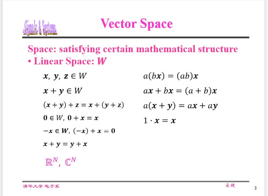
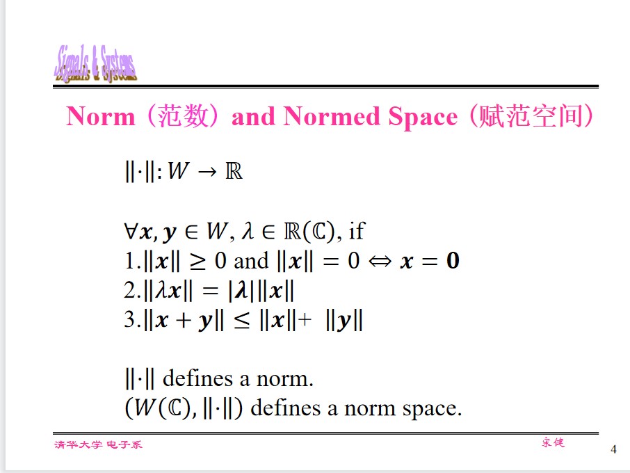
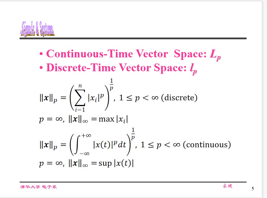
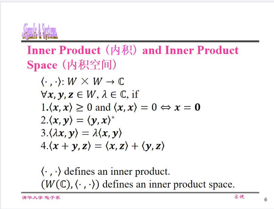
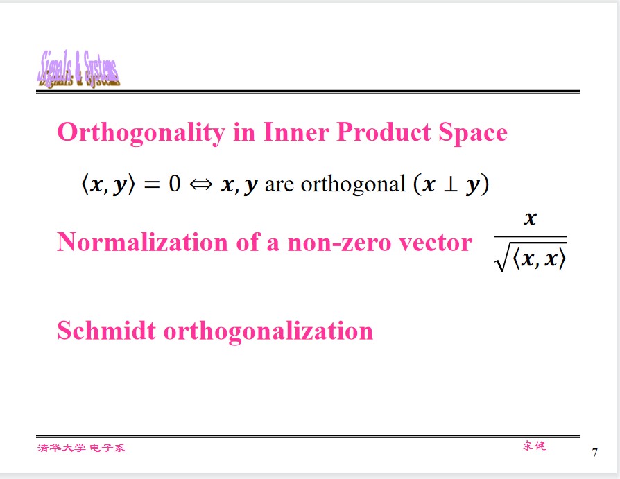
Objective for singal decomposition
$$ r(t) = H[e(t)] = H\left[\sum_{i=0}^ne_i(t)\right] = \sum_{i=0}^nH[e_i(t)] $$Basics
Orthogonal Vector
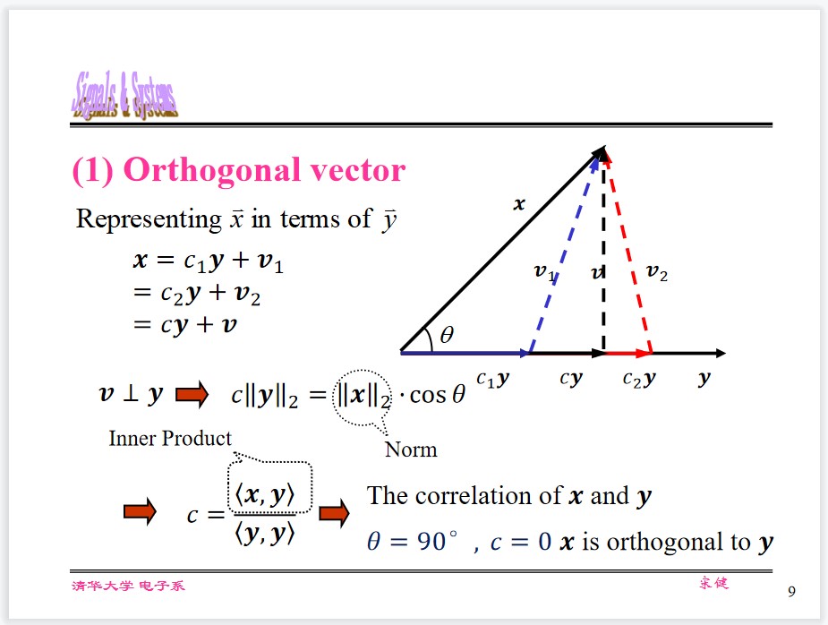
Orthogonal Function
Represend $f_1(t)$ in terms of $f_2(t)$ (both real), for $t_1<t<t_2$
$$ f_1(t)\approx c_{12}f_2(t) $$Residual error $\overline{\varepsilon^2} = \overline{f_e^2(t)} = \frac{1}{t_2 - t_1}\int_{t_1}^{t_2}[f_1(t) - c_{12}f_2(t)]^2\mathrm dt$
Let $\frac{\mathrm d \overline{\varepsilon^2}}{\mathrm d c_{12}} = 0$ , then $\overline{\varepsilon^2}$ is minimized.
The coefficient can be determined as
$$ c_{12} = \frac{\int_{t_1}^{t_2}f_1(t)f_2(t)\mathrm dt}{\int_{t_1}^{t_2}f_2^2(t)\mathrm dt} = \frac{\langle f_1, f_2\rangle}{\langle f_2, f_2\rangle} $$If $c_{12} = 0$ , then $f_1(t), f_2(t)$ are called Orthogonal Functions.
And
$$ \int_{t_1}^{t_2}f_1(t)f_2(t)\mathrm dt = 0 $$Orthogonal Function Set
Any real function $f(t)$ can be represented as the sum of $n$ -D orthogonal real functions.
$$ f(t) = \sum_{r=1}^n c_rg_r(t) $$According to the minimal mean square error, the coefficient can be determined as
$$ c_r = \frac{\int_{t_1}^{t_2}f(t)g_r(t)\mathrm dt}{\int_{t_1}^{t_2}g_r^2(t)\mathrm dt} = \frac{\langle f, g_r\rangle}{\langle g_r, g_r\rangle} $$If $g_1(t), g_2(t), ..., g_n(t)$ are orthogonal to each other, i.e.
$$ \int_{t_1}^{t_2}g_r(t)g_s(t)\mathrm dt =\begin{cases} K_i, &r = s,\\ 0, &r \ne s \end{cases} $$Then $f(t)$ can be represented as the sum of $n$ -D orthogonal real functions.
Then $g_1(t), g_2(t), ..., g_n(t)$ are called Orthogonal Function Set.
If $\int_{t_1}^{t_2}g_i^2(t)\mathrm dt = 1$ , the orthogonal function set is called Orthonormal Function Set.
Orthogonality of Complex Function
$$ c_{12} = \frac{\int_{t_1}^{t_2}f_1(t)f_2^*(t)\mathrm dt}{\int_{t_1}^{t_2}f_2(t)f_2^*(t)\mathrm dt} = \frac{\langle f_1, f_2^*\rangle}{\langle f_2, f_2^*\rangle} $$Orthogonal Function Set satisfies
$$ \int_{t_1}^{t_2}g_r(t)g_s^*(t)\mathrm dt =\begin{cases} K_i, &r = s,\\ 0, &r \ne s \end{cases} $$The definition of Orthogonal is
$$ \int_{t_1}^{t_2}f_1(t)f_2^*(t)\mathrm dt = \int_{t_1}^{t_2}f_2(t)f_1^*(t)\mathrm dt = 0 $$NOTE:
If two signals are orthogonal within a given interval, they are not necessarily orthogonal within other intervals.
If two signals are not orthogonal, they must be correlated.
Complete Orthogonal Function and Parseval’s Theorem
Complete Orthogonal Funtion Set
$$ \overline{\varepsilon^2} = \frac{1}{t_2-t_1}\left[\int_{t_1}^{t_2}f^2(t)\mathrm dt - \sum_{r = 1}^nc_r^2K_r\right] $$If $\lim_{t_2 \to \infty}\overline{\varepsilon^2} = 0$ , then $\{g_r(t)\}$ is said to be a Complete Orthogonal Function Set.
Alternative definition of complete orthogonal set
Other than the elements in $\{g_r(t)\}$ , there is no finite-energy signal $x(t)$ , which satisfies
$$ \int_{t_1}^{t_2}x(t)g_r(t)\mathrm dt = 0, \forall r\\ \text{or } \int_{t_1}^{t_2}x(t)g_r^*(t)\mathrm dt = 0, \forall r $$Trigonometric Set
$$ \left\{\cos n\omega_1 t\right\}_{n\rightarrow\infty}\\ \left\{\sin n\omega_1 t\right\}_{n\rightarrow\infty} $$Complex exponential set
$$ \left\{e^{jn\omega_1 t}\right\}_{n\rightarrow\infty} $$Parseval’s Theorem
$$ \int_{t_1}^{t_2}f(t)^2\mathrm dt = \sum_{r=1}^\infty c_r^2K_r = \sum_{r=1}^\infty\int_{t_1}^{t_2}[c_rg_r(t)]^2\mathrm dt $$Physical interpretation:
The energy (power) of a signal always equals to the sum of the energy (power) of all its components in a complete orthogonal function set.
Mathematical interpretation:
The norm of vector signals keeps invariant under orthogonal transform.
Correlation
Physical interpretation:
Gauge of the similarity of two signals
Energy and Power Signals
Instaneous Power $p(t) = i^2(t) R$
The energy consumed by $R$ in a period
$$ E = \int_{-T_0/2}^{T_0/2}p(t)\mathrm dt = R\int_{-T_0/2}^{T_0/2}i^2(t) \mathrm dt $$Average Power:
$$ P = \frac{1}{T_0}\int_{-T_0/2}^{T_0/2}p(t)\mathrm dt = \frac{1}{T_0}R\int_{-T_0/2}^{T_0/2}i^2(t) \mathrm dt $$The energy signals and power signals:
$$ E = \lim_{T_0 \to \infty}\int_{-T_0/2}^{T_0/2}f^2(t)\mathrm dt\\ P = \lim_{T_0 \to \infty}\frac{1}{T_0}\int_{-T_0/2}^{T_0/2}f^2(t)\mathrm dt $$Correlation Coefficient
$$ \rho_{12} = \frac{\int_{t_1}^{t_2}f_1(t)f_2^*(t)\mathrm dt}{\sqrt{\int_{t_1}^{t_2}f_1^2(t)\mathrm dt}\sqrt{\int_{t_1}^{t_2}f_2^2(t)\mathrm dt}} = \frac{\langle f_1, f_2\rangle}{\sqrt{\langle f_1, f_1\rangle}\sqrt{\langle f_2, f_2\rangle}} = \frac{\langle f_1, f_2\rangle}{\|f_1\|_2\|f_2\|_2} $$If $f_1(t)$ is a linear function of $f_2(t)$ , then $\rho_{12} = \pm1$ , $\overline{\varepsilon^2} = 0$ .
If $f_1(t)$ is orthogonal to $f_2(t)$ , then $\rho_{12} = 0$ , $\overline{\varepsilon^2}$ is maximized.
- Describe the correlation of two signals from the perspective of energy difference.
- Quantitatively measure the correlation of two signals in terms of inner product.
Correlation Function
The similarity between one signal with a delayed version of another signal.
(1) $f_1(t)$ and $f_2(t)$ are both real and energy signals
$$ R_{12}(\tau) = \int_{-\infty}^{\infty}f_1(t)f_2(t-\tau)\mathrm dt = \int_{-\infty}^{\infty}f_1(t + \tau)f_2(t)\mathrm dt\\ R_{21}(\tau) = \int_{-\infty}^{\infty}f_2(t)f_1(t-\tau)\mathrm dt = \int_{-\infty}^{\infty}f_2(t + \tau)f_1(t)\mathrm dt\\ R_{12}(\tau) = R_{21}(-\tau) $$(2) $f_1(t)$ and $f_2(t)$ are both complex and energy signals
If $f_1(t) = f_2(t) = f(t)$
Autocorrelation:
$$ R(\tau) = \int_{-\infty}^{\infty}f(t)f(t-\tau)\mathrm dt = \int_{-\infty}^{\infty}f(t + \tau)f(t)\mathrm dt\\ $$(2) $f_1(t)$ and $f_2(t)$ are both complex and energy signals
$$ R_{12}(\tau) = \int_{-\infty}^{\infty}f_1(t)f_2^*(t-\tau)\mathrm dt = \int_{-\infty}^{\infty}f_1(t + \tau)f_2^*(t)\mathrm dt\\ R_{21}(\tau) = \int_{-\infty}^{\infty}f_2(t)f_1^*(t-\tau)\mathrm dt = \int_{-\infty}^{\infty}f_2(t + \tau)f_1^*(t)\mathrm dt\\ R_{12}(\tau) = R_{21}^*(-\tau) $$Autocorrelation:
$$ R(\tau) = \int_{-\infty}^{\infty}f(t)f^*(t-\tau)\mathrm dt = \int_{-\infty}^{\infty}f(t + \tau)f^*(t)\mathrm dt\\ R(\tau) = R^*(-\tau) $$(3) $f_1(t)$ and $f_2(t)$ are both real and power signals
$$ R_{12}(\tau) = \lim_{T\rightarrow\infty}\left[\frac1T\int_{-T/2}^{T/2}f_1(t)f_2(t-\tau)\mathrm dt \right]\\ R_{21}(\tau) = \lim_{T\rightarrow\infty}\left[\frac1T\int_{-T/2}^{T/2}f_2(t)f_1(t-\tau)\mathrm dt \right]\\ $$Autocorrelation
$$ R(\tau) = \lim_{T\rightarrow\infty}\left[\frac1T\int_{-T/2}^{T/2}f(t)f(t-\tau)\mathrm dt \right]\\ $$(4) $f_1(t)$ and $f_2(t)$ are both complex and power signals
$$ R_{12}(\tau) = \lim_{T\rightarrow\infty}\left[\frac1T\int_{-T/2}^{T/2}f_1(t)f_2^*(t-\tau)\mathrm dt \right]\\ R_{21}(\tau) = \lim_{T\rightarrow\infty}\left[\frac1T\int_{-T/2}^{T/2}f_2(t)f_1^*(t-\tau)\mathrm dt \right]\\ $$Autocorrelation
$$ R(\tau) = \lim_{T\rightarrow\infty}\left[\frac1T\int_{-T/2}^{T/2}f(t)f^*(t-\tau)\mathrm dt \right]\\ $$Correlation Theorem
$$ \mathcal F(x(t)) = X(\omega)\\ \mathcal F(y(t)) = Y(\omega)\\ \mathcal F(R_{xy}(\tau)) = X(\omega)Y^*(\omega)\\ $$If $x(t) = y(t)$ , The FT of the autocorrelation function is $\mathcal F[{R_{xx}(\tau)}] = |X(\omega)|^2$
If $y(t)$ is a real and even function: $Y^*(\omega) = Y(\omega)$
Then the correlation theorem is equivalent to the convolution theorem
$$ \mathcal F(\int_{-\infty}^\infty x(t)y(t-\tau)\mathrm dt) = X(\omega)Y(\omega)\\ $$Generally,
$$ R_{12}(t) = f_1(t) * f_2(-t) $$Energy & Power Spectral Density
$$ R(\tau) = \int_{-\infty}^{\infty}f(t)f^*(t-\tau)\mathrm dt\\ $$ $$ R(\tau) = \frac{1}{2\pi}\int_{-\infty}^{\infty}\lvert F(\omega)\rvert^2 e^{j\omega\tau}\mathrm d\omega\\ |F(\omega)|^2 = \int_{-\infty}^{\infty}R(\tau)e^{-j\omega\tau}\mathrm d\tau\\ $$ $$ R(0) = \int_{-\infty}^{\infty}f(t)f^*(t)\mathrm dt = \int_{-\infty}^{\infty}\lvert f(t)\rvert^2\mathrm dt\\ R(0) = \frac{1}{2\pi}\int_{-\infty}^{\infty}\lvert F(\omega)\rvert^2\mathrm d\omega\\ $$ $$ \int_{-\infty}^{\infty}\lvert f(t)\rvert^2\mathrm dt = \frac{1}{2\pi}\int_{-\infty}^{\infty}\lvert F(\omega)\rvert^2\mathrm d\omega $$Energy Spectral Density
$$ \mathcal{E}(\omega) = \lvert F(\omega)\rvert^2\\ $$ $$ \mathcal{E}(\omega) = \mathcal{F}[R(\tau)]\\ R(\tau) = \mathcal{F}^{-1}[\mathcal{E}(\omega)]\\ $$Power Spectral Density
$$ \mathcal F[ R(\tau)] = \mathcal P(\omega)\\ $$It is called Power Spectral Density (PSD).
Wiener-Khinchin Theorem
$$ R(\tau) = \frac{1}{2\pi}\int_{-\infty}^{\infty}\mathcal P(\omega)e^{j\omega\tau}\mathrm d\tau\\ \mathcal P(\omega) = \int_{-\infty}^{\infty}R(\tau)e^{-j\omega\tau}\mathrm d\omega\\ $$ESD/PSD of the System Response
$$ |R(j\omega)|^2 = |H(j\omega)|^2|E(j\omega)|^2\\ \mathcal{E}_r(\omega) = |H(j\omega)|^2\mathcal{E}_e(\omega)\\ \mathcal{P}_r(\omega) = |H(j\omega)|^2\mathcal{P}_e(\omega)\\ $$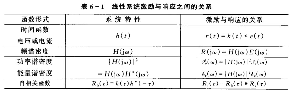
The last line of this table is wrong. The correct is:
$$ R_h(\tau) = h(\tau) * h^*(-\tau) $$Match Filters
$$ H(j\omega) = kS(-j\omega)e^{-j\omega t_m}\\ h(t) = ks(t_m - t)\\ $$ $t_m$ is the signal width in TD.Discrete time signals
Discrete time-axis, but continuous amplitude-axis
Sequence operation
Addition $z(n) = x(n) + y(n)$
Multiplication $z(n) = x(n) * y(n)$
Multiplied a coefficient $z(n) = a * x(n)$
Shift $z(n) = x(n - m)$ right shift( $m>0$ ), $z(n) = x(n +m)$ left shift
Reflection $z(n) = x(-n)$
Difference $\Delta x(n) = x(n + 1) - x(n)$ Forawrd difference,
$\nabla x(n) = x(n) - x(n - 1)$ Backward difference $\nabla^mx(n) = \nabla(\nabla^{m-1}x(n))$Summation $z(n) = \sum_{k = -\infty}^{n}x(k)$
Scaling $z(n) = z(2n)$ squeeze,
$z(n) = x(n/2)$ , extendTypical sequences
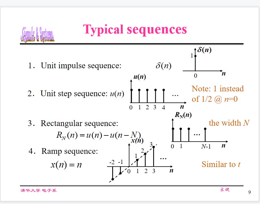
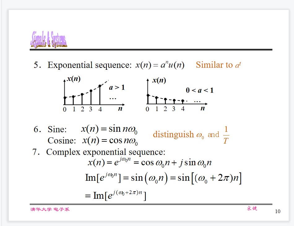
Relations of several singal waveforms
$$ u(n) = \sum_{k = 0}^{\infty}\delta(n - k)\\ \delta(n) = u(n) - u(n - 1)\\ R_N(n) = u(n) - u(n - N)\\ $$Signal Decomposition
$$ x(n) = \sum_{m = -\infty}^{\infty}x_m\delta(n - m)\\ $$ $$ \delta(n - m) = \begin{cases} 1, & n = m\\ 0, & n \neq m \end{cases} $$Difference equations
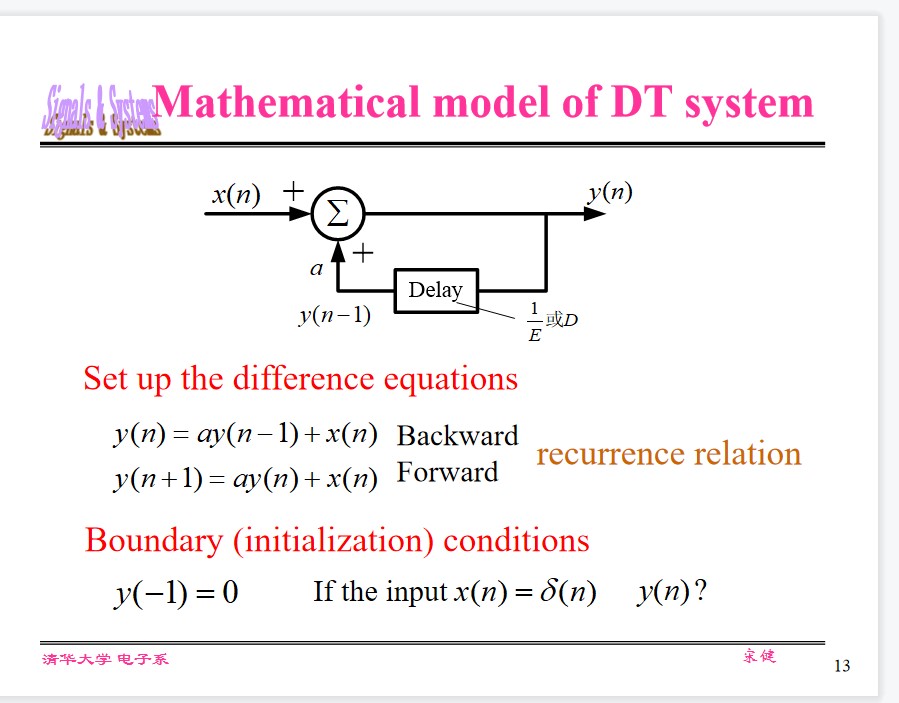
Numerical solution of difference equations
General form of difference equation:
$$ \sum_{k = 0}^N a_ky(n - k) = \sum_{r = 0}^M b_ry(n - r)\\ $$Methods:
- Recursive method
- Intuitive, difficult to formulate the closed-form solutions
- Time-domain classical method
- Obtain homogeneous and particular solutions and using the boundary condition to determine the coefficients.
- The sum of the zero-input and zero-state responses
- Convolution (next class)
- Z-transform (Chapter 8)
- State variable method (Chapter 11)
Homogeneous Solution
$$ \sum_{k = 0}^N a_ky(n - k) = 0\\ $$The characteristic root $\alpha_k$ satisfies:
$$ a_0\alpha^N + a_1\alpha^{N-1} + \cdots + a_N = 0\\ $$The homogeneous solution is:
$$ y(n) = c_1\alpha_1^n + c_2\alpha_2^n + \cdots + c_N\alpha_N^n\\ $$Particular Solutions:
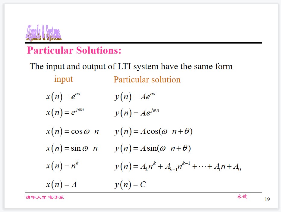
General steps
- Obtain homogeneous solutions from characteristic equation $c_1\alpha_1^n + c_2\alpha_2^n + \cdots + c_N\alpha_N^n$
- Determine the form of the particular solution $D(n)$
- The complete solution $c_1\alpha_1^n + c_2\alpha_2^n + \cdots + c_N\alpha_N^n + D(n)$
- Introduce the boundary condition and set up equations $$ y(0) = C_1 +C_2 + \cdots + C_N + D(0)\\ y(1) = C_1\alpha_1 +C_2\alpha_2 + \cdots + C_N\alpha_N + D(1)\\ \vdots\\ y(N - 1) = C_1\alpha_1^{N - 1} + C_2\alpha_2^{N - 1} + \cdots + C_N\alpha_N^{N - 1} + D(N - 1)\\ \Rightarrow\\ Y(k) - D(k) = VC\\ C = V^{-1}(Y(k) - D(k))\\ $$
Zero-input and zero-state responses
$$ y(k) = y_{zi}(k) + y_{zs}(k) $$Zero-Input Response
$D(k) = 0 \Rightarrow C_{zi} = V^{-1}Y_{zi}(k)$Zero-State Response
$$ \begin{align*} C_{zs} &= V^{-1}[Y_{zs}(k) - D(k)]\\ C_{zs} &= V^{-1}[Y(k) - Y_{zi}(k) - D(k)]\\ C &= C_{zi} + C_{zs}\\ \end{align*} $$Natural Response $\sum_{k = 1}^NC_k\alpha_k^n$
Forced Response $D(n)$
Characteristics of the boundary condition for difference equations
N-th order difference equation should have N independent boundary conditions.
Compared with continuous systems, there are no big differences between $0_+$ and $0_-$ in discrete systems.
$y(-1), y(-2), \dots, y(-N)$ are the system memory (storage) before the excitation is added: $0_-$Derive (together with the excitation) $y(0), y(1), …, y(N-1): 0_+$
Using Z-transform can avoid mistakes-similar to the Laplace transform in continuous systems.
Impulse response of DT systems
Similar to CT System, h(n) reflects system’s property
Causality $h(n) = h(n) u(n)$ (unlateral, $n\lt 0$ no response)
Stability $\sum_{n=-\infty}^\infty |h(n)| \lt \infty$ (absolutely summable)
NOTE: critical stability can be considered as either stable or unstable, e.g., system whose impulse response is a sine sequence
Not all practical discrete systems are necessarily causal:
- Variable is not time, like image processing
- Variable is time, but data has been recorded and processed, like voice processing, meteorology, stock systems.
Example: Smooth windowing
$$ y(n) = \frac{1}{2M+1}\sum_{k=-M}^M x(n-k) $$Discrete non-causal system
Convolution Sum
$$ y(n) = \sum_{m = -\infty}^\infty x(m)h(n - m) = h(n) * x(n) $$Similar to CT system, also satisfies both distributive and associative laws
Calculation of convolution:
Four steps: reflection, shift, multiplication and summation.
Calculation of correlation:
Cross- & auto-correlation: shift, multiplication & summation.
Example:
$$ x(n) = u(n) - u(n - N)\\ h(n) = a^nu(n)\\ y(n) = x(n) * h(n) $$ $$ y(n) = \sum_{m = -\infty}^\infty [u(m) - u(m - N)]a^{n - m}u(n - m) $$if $n < 0$ , then $y(n) = 0$
if $0 \le n \lt N - 1$ , $y(n) = \sum_{m = 0}^na^{n-m} = \frac{1}{1 - a}[1 - a^{n+1}]$
if $n \ge N - 1$ , $y(n) = \frac{1 - a^{-N}}{1 - a^{-1}}a^n$
Deconvolution
Signal retrieval y(n) and h(n) are known, how to derive x(n)?
Measurement equipment (linear system), like sensor for measuring blood pressure
System identification y(n) and x(n) are known, how to derive h(n)?
Earthquake signal, like geological survey, oil exploration, etc.
$$ \begin{bmatrix*} y(0)\\ y(1)\\ y(2)\\ \vdots\\ y(n) \end{bmatrix*} = \begin{bmatrix*} h(0) & 0 & 0 & \dotsb & 0\\ h(1) & h(0) & 0 & \dotsb & 0\\ h(2) & h(1) & h(0) & \dotsb & 0\\ \vdots & \vdots & \vdots & \ddots & \vdots\\ h(n) & h(n-1) & h(n-2) & \dotsb & h(0)\\ \end{bmatrix*}\begin{bmatrix*} x(0)\\ x(1)\\ x(2)\\ \vdots\\ x(n) \end{bmatrix*} $$Thus,
$$ x(n) = \left[y(n) - \sum_{m = 0}^{n-1} x(m) h(n - m)\right]/h(0)\\ h(n) = \left[y(n) - \sum_{m = 0}^{n-1} h(m) x(n - m)\right]/x(0) $$Important Concepts

- Symbol rate : clock period is $T$ , signal symbol rate is $f = 1/T$ .
- Information rate: information rate equals to symbol rate for binary encoding, otherwise, equal to multiplication between symbol rate and number of information bits per symbol.
- Signal bandwidth: the first zero of non-return-to-zero (NRZ) signal’s spectrum is $1/T$ , so the signal bandwidth is $B=1/T =f$ .
这句话是在介绍非归零码(Non-Return-to-Zero,简称NRZ)信号的带宽计算方式。
在信号处理和通信中,信号的频谱表示了信号在不同频率上的能量分布。对于一个NRZ信号,它的频谱图中第一个零点(也就是在零周围出现的第一个极小值点)出现在频率为 $1/T$ 处,其中 $T$ 是NRZ信号中一个脉冲的时间长度。这是因为NRZ信号的频谱是由一个周期为 $T$ 的方波产生的,其频率成分只包含正弦函数的奇次谐波。其中,最低的一个谐波频率是 $f=\frac{1}{T}$ ,对应的是频率为 $f$ 的正弦波。所以,NRZ信号的带宽 $B$ 就被定义为 $f=1/T$ 。
简而言之,NRZ信号的带宽是由脉冲的时间长度决定的,具体来说,带宽等于脉冲频率的一半,即带宽等于 $f=1/T$ 。
NOTE:
When NRZ code is used, signal bandwidth = symbol rate
When return-to-zero (RZ) code is used, signal bandwidth > symbol rate
Using NRZ code can save bandwidth yet high frequency components of the rectangular signal will suffer from the severe inter-symbol interference (ISI). So the raised cosine or Sa function is preferred.
ChatGPT:
归零码和非归零码都是数字通信中常用的编码方式。
归零码(Return-to-Zero,简称RZ)是一种二进制码,其中一个信号所代表的位是由一个脉冲表示的。发送二进制“1”时,脉冲电平为高电平,发送二进制“0”时,脉冲电平为低电平。在归零码中,一个信号位所代表的脉冲之后,信号在下一时刻会回到零电平。由于归零码中每个脉冲结束时信号回到零电平,因此这种编码方式具有稳定可靠的特点,但是传输的带宽相对较大。
非归零码(Non-Return-to-Zero,简称NRZ)的编码方式与归零码不同之处在于,在NRZ信号中,一个信号所代表的位是由一个固定电平表示的。当信号所代表的位是二进制“1”时,固定电平为高电平;当信号所代表的位是二进制“0”时,固定电平为低电平。这种编码方式的好处是带宽更小,但是却存在着在多个二进制“1”连续发送时,出现误解的情况。
综上所述,归零码是二进制码中脉冲与幅度的双重编码,不易产生传输误码,但其对于通信带宽需求较大;而非归零码不需要对脉冲进行编码,在带宽方面具有一定的优势,但长时间连续发送相同信息时会产生误解。
Z-Transform
Similar to the L-Tranform.
Definition
$$ X(z) = Z(x(n)) = \sum_{n = -\infty}^{\infty} x(n) z^{-n} $$Z-T of Typical Series
$z \in \Complex$ $$ \delta(n) \rightarrow 1\\ u(n) \rightarrow \frac{1}{1-z^{-1}}(|z| \gt 1)\\ nu(n) \rightarrow \frac{z^{-1}}{(1-z^{-1})^2}(|z| \gt 1)\\ a^n u(n) \rightarrow \frac{1}{1-az^{-1}}(|z| \gt |a|)\\ \cos(\omega_0 n) u(n) \rightarrow \frac{1-z^{-1}\cos(\omega_0)}{1-2z^{-1}\cos(\omega_0) + z^{-2}}\\ \sin(\omega_0 n) u(n) \rightarrow \frac{z^{-1}\sin(\omega_0)}{1-2z^{-1}\cos(\omega_0) + z^{-2}}\\ $$The Region of Convergence
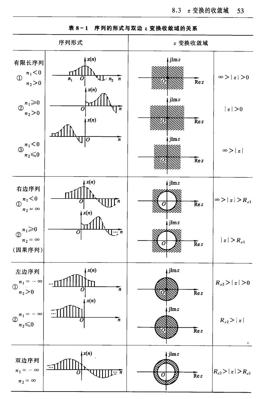
Inverse Z-Transform
$$ x(n) = \frac{1}{2\pi j} \oint_C X(z) z^{n-1} dz $$Method
Contour Integration(residue method)
Right-sided sequence
$$ x(n) = \sum_{k = 1}^{N} Res\{X(z)z^{n-1}\}|_{z = z_k} $$Left-sided sequence
$$ x(n) = - \sum_{k = 1}^{N} Res\{X(z)z^{n-1}\}|_{z = z_k} $$Power series expansion(Long division)
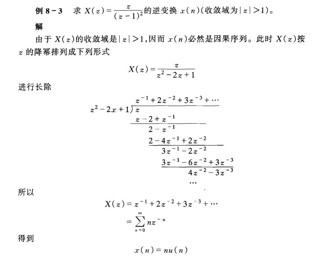
If it is right sided,
$$ X(z) = \sum_{n = 0}^\infty x(n)z^{-n} $$If it is left sided,
$$ X(z) = \sum_{n = -\infty}^{-1}x(n)z^{-n} $$Partial Fraction Expansion
$$ \frac{z}{z - a} \lrarr \begin{cases} a^nu(n), &|z|\gt |a|\\ -a^nu(-n-1), &|z|\lt |a| \end{cases} $$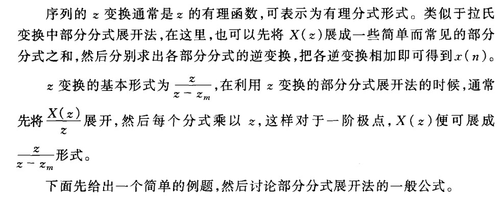
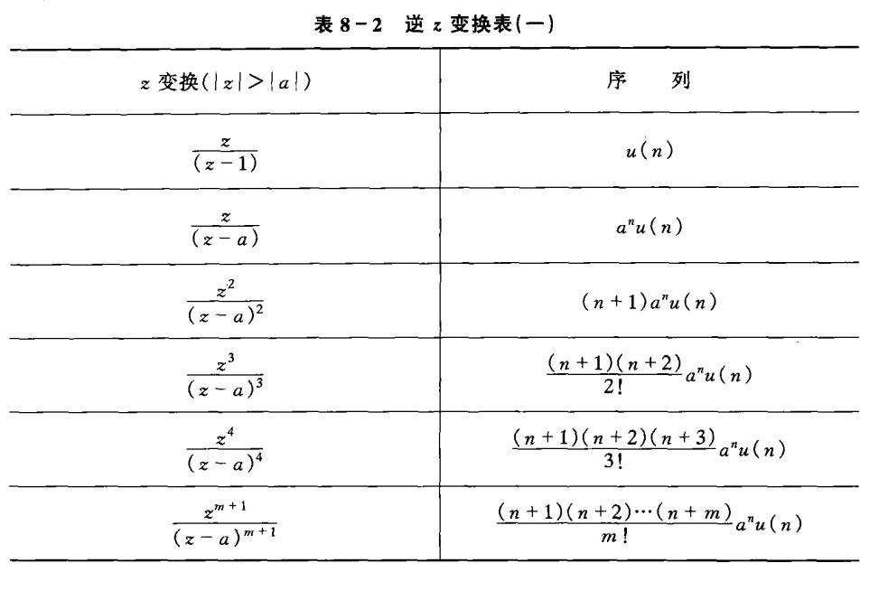
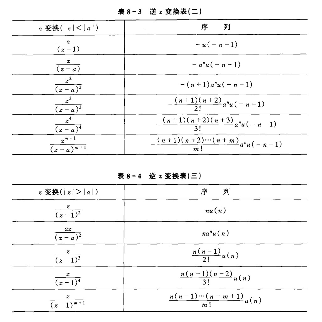
Properties of Z-T
Linearity
Addition and homogeneity
ROC may change!
i.e. poles are cancelled when added: ROC will enlarge or and shrink.
Time shifting
(a) bilateral: If $\mathcal Z[x(n)] = X(z), R_{X_1} < |z| < R_{X_2}$ , then $\mathcal{Z}[x(n-m)] = z^{-m}X(z), R_{X_1} < |z| < R_{X_2}$ .
(b) unilateral: if $\mathcal{Z}[x(n)] = X(z), R_{X_1} < |z|$ , then $\mathcal{Z}[x(n-m)] = z^{-m}[X(z) + \sum_{k = -m}^{-1}x(k)z^{-k}], R_{X_1}\lt |z|$ , and $\mathcal{Z}[x(n+m)] = z^{m}[X(z) - \sum_{k = 0}^{m-1}x(k)z^{-k}], R_{X_1}\lt |z|$
For casual sequence, $n < 0, x(n) = 0$ , the unilateral is also $\mathcal{Z}[x(n-m)] = z^{-m}X(z)$ .
The reason is that the unilateral z transform doesn’t contain the $n<0$ parts of sequence, but after shifting, sometimes must be counted(right shift), sometimes must be discarded(left shift).
Linear weighting on sequence(Z domain differentiation)
$$ \mathcal{Z}[x(n)] = X(z) \Rightarrow nx(n)\lrarr -z\frac{dX(z)}{dz} $$Generalization:
$$ n^mx(n)\lrarr \bigg[-z\frac{d}{dz}\bigg]^m X(z) $$Geometric progression(Z-domain scaling)
$$ a^n(x^n) \lrarr X(\frac{z}{a})\\ (R_{x1} \lt \bigg|\frac{z}{a}\bigg| \le R_{x2}) $$ $$ a^{-n}x(n) \lrarr X(az)\\ (-1)^nx(n) \lrarr X(-z) $$Initial-value theorem
$$ x(0) = \lim_{z \rightarrow \infty }X(z) $$Final-value theorem
$$ \lim_{n \rightarrow \infty } x(n) = \lim_{z \rightarrow 1}[(z-1)X(z)] $$condition: when $n \rightarrow \infty$ , $x(n)$ converge
Thus, the poles of $X(z)$ are inside the unit circle, the radius of ROC is less than 1.
For $a^nu(n), |a| \lt 1$ , the final value is 0.
Or, if the pole is on the unit circle, it should be 1, and is of the 1st order.
$u(n)$ 's final value is 1.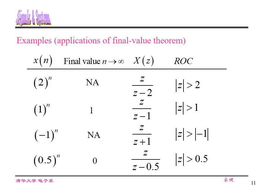
Time-domain convolution theorem
If $\mathcal{Z}{x(n)} = X(z), (R_{x1} \lt |z| \lt R_{x2}), \mathcal{Z}{h(n)} = H(z), (R_{h1} \lt |z| \lt R_{h2})$
$$ \mathcal{Z}[x(n) * h(n)] = X(z)H(z)\\ \max(R_{x1}, R_{h1}) \lt |z| \lt \min(R_{x2}, R_{h2}) $$If poles are cancelled in multiplication, ROC is enlarged.
Conclusion: (Z Transform) convolution in time-domain is equivalent to multiplication (of Z Transform) in Z-domain.
Z domain convolution theorem
$$ \mathcal{Z}[x(n)h(n)] = \frac{1}{2\pi j} \oint_C X(\frac{z}{v})H(v)v^{-1}dv $$or
$$ \mathcal{Z}[x(n)h(n)] = \frac{1}{2\pi j} \oint_C X(v)H(\frac{z}{v})v^{-1}dv $$where $C$ is a closed contour in the intersection of ROCs of $X(\frac{z}{v})$ and $H(v)$ or $X(v)$ and $H(\frac z v)$ .
let $v = \rho e^{j\theta}, z = r e^{j\varphi}$ ,
then
$$ \mathcal Z[x(n)h(n)] = \frac{1}{2\pi}\int_{-\pi}^\pi X(\rho e^{j\theta})H(\frac r\rho e^{-j(\varphi - \theta)})d\theta $$Mapping of ZT and LT
$$ z = e^{sT} ,\omega_s = \frac{2\pi}{T} \\ re^{j\theta} = e^{(\sigma + j\omega)T}\\ $$then,
$$ r = e^{\sigma T} = e^{2\pi\frac{\sigma}{\omega_s}}\\ \theta = \omega T = 2\pi\frac{\omega}{\omega_s} $$when $\sigma$ is constant,
vertical line in $s$ -plane maps the circle in $z$ -plane.
$s$ -plane imaginary axis maps the unit circle in $z$ -plane.when $\omega$ is constant,
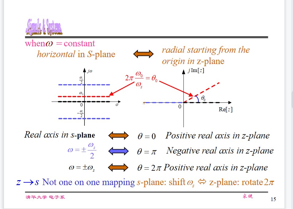
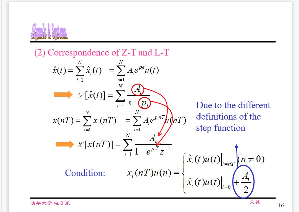
Correspondence of ZT and LT
Solving difference equation by Z-T
$$ \sum_{k = 0}^N a_ky(n-k) = \sum_{r = 0}^M b_rx(n-r) $$Two methods:
- TD method
- Z-T method (notice the ROC)
ZT method
- perform unilateral Z-T on both sides.
- Derive $Y(z)$
- Perform inverse transform on $Y(z)$ to get $y(n)$ (ROC!)
Zero input response
$$ x(n) = 0\\ Y(z) = \frac{-\sum_{k = 0}^M[a_kz^{-k}\cdot \sum_{l = -k}^{-1}y(l)z^{-l}]}{\sum_{k = 0}^Na_kz^{-k}} $$Zero state response
$$ y(l) = 0\\ \text{ casual sequence }: x(m) = 0\\ \sum_{k = 0}a_kz^{-k}Y(z) = \sum_{r = 0}^M b_rz^{-r}X(z)\\ Y(z) = X(z)\cdot\frac{\sum_{r = 0}^M b_rz^{-r}}{\sum_{k = 0}^Na_kz^{-k}} = X(z)\cdot H(z) $$System function of DT system
Unit Impulse/sample response $h(n)$ and system function H(z)
$$ y(n) = x(n) * h(n)\\ Y(z) = H(z)\cdot X(z) $$ $$ H(z) = \frac{Y(z)}{X(z)} = \frac{\sum_{r = 0}^M b_rz^{-r}}{\sum_{k = 0}^Na_kz^{-k}} $$Factorization
$$ H(z) = \frac{\prod_{r = 1}^M(1-z_rz^{-1})}{\prod_{k=1}^N1-p_kz^{-1}} $$We can draw the conclusions directly from the relationship between Z-T and L-T
| Imaginary axis | $\sigma=0$ | Constant amplitude | $r = 1$ | Unit circle |
| Right half plane | ||||
| Left half plane | ||||
| Real axis |

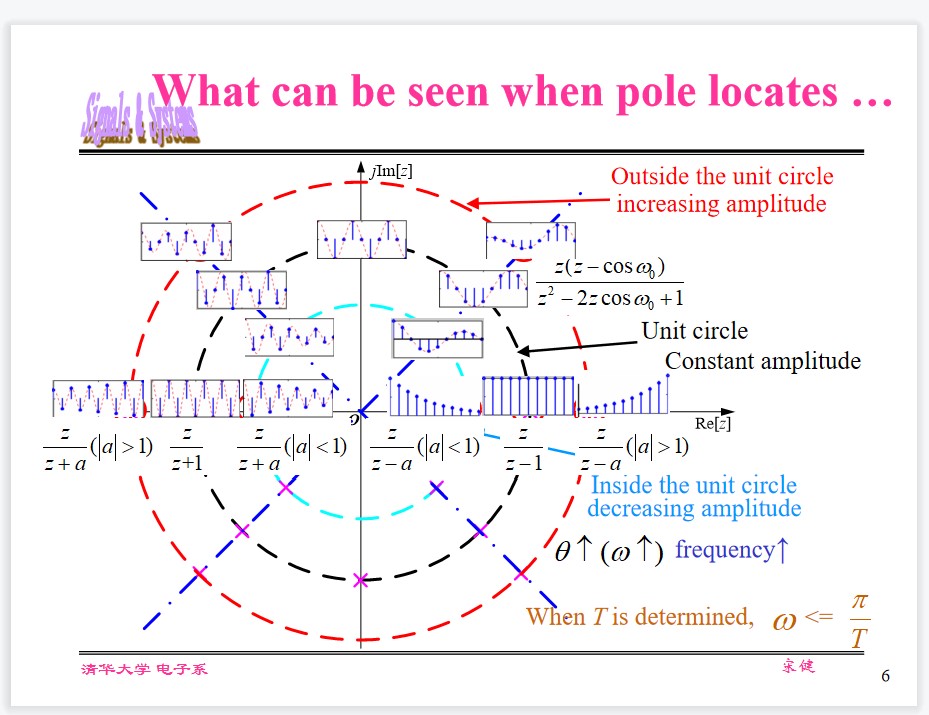
Stability and Causality
Stable: iff
$$ \sum_{n=-\infty}^\infty |h(n)|\lt \infty $$ $$ z = 1, H(z) = \sum_{n=-\infty}^\infty h(n)\lt \infty $$The condition is ROC of stable system includes the unit circle.
Causal:
$$ h(n) = h(n)u(n) $$Condition is ROC includes $\infty$ : $R_{X_1}\lt |z|$
Stable and causal
$$ a\le |z| \le \infty, a\le 1 $$Discrete-time Fourier Transform(DTFT)
Definition
$$ \mathcal{F}[x(t)\delta_T(t)] = \int_{-\infty}^\infty x(t)\delta_T(t)e^{-j\omega t}dt = \sum_{n=-\infty}^\infty x(nT)e^{-j\omega nT} $$take $T = 1$
$$ \sum_{n=-\infty}^\infty x(n)e^{-j\omega n} = \text{DTFT[x(n)]} $$The relation ship with Z-T:
$$ X(z) = \sum_{n = -\infty}^\infty x(n)z^{-n}, z = e^{j\omega}\\ $$ $$ DTFT[x(n)] = X(z)|_{|z|=1} = X(z)|_{z = e^{j\omega}} = X(e^{j\omega}) $$Inverse transform
$$ x(n) = \frac{1}{2\pi j}\oint_{|z| = 1}X(z)z^{n-1}\mathrm dz=\frac{1}{2\pi}\int_{-\pi}^\pi X(e^{j\omega})e^{j\omega n}\mathrm d\omega $$Frequency Response of DT system
The steady-state response to sine sequence
$$ x(n) = A\sin(n\omega)(n\ge 0)\\ y_{ss}(n) = A|H(e^{j\omega})|\sin(n\omega + \varphi)\\ H(e^{j\omega}) = \sum_{n=-\infty}^\infty h(n)e^{-jn\omega} $$The FT of $h(n)$ , $H(e^{j\omega})$ is a periodic function with period of $\omega_s = 2\pi /T = 2\pi$ .
If $h(n)$ is real, then the amplitude/phase response is even/odd function.
The amplitude is determined within $[0, \omega_s/2]$
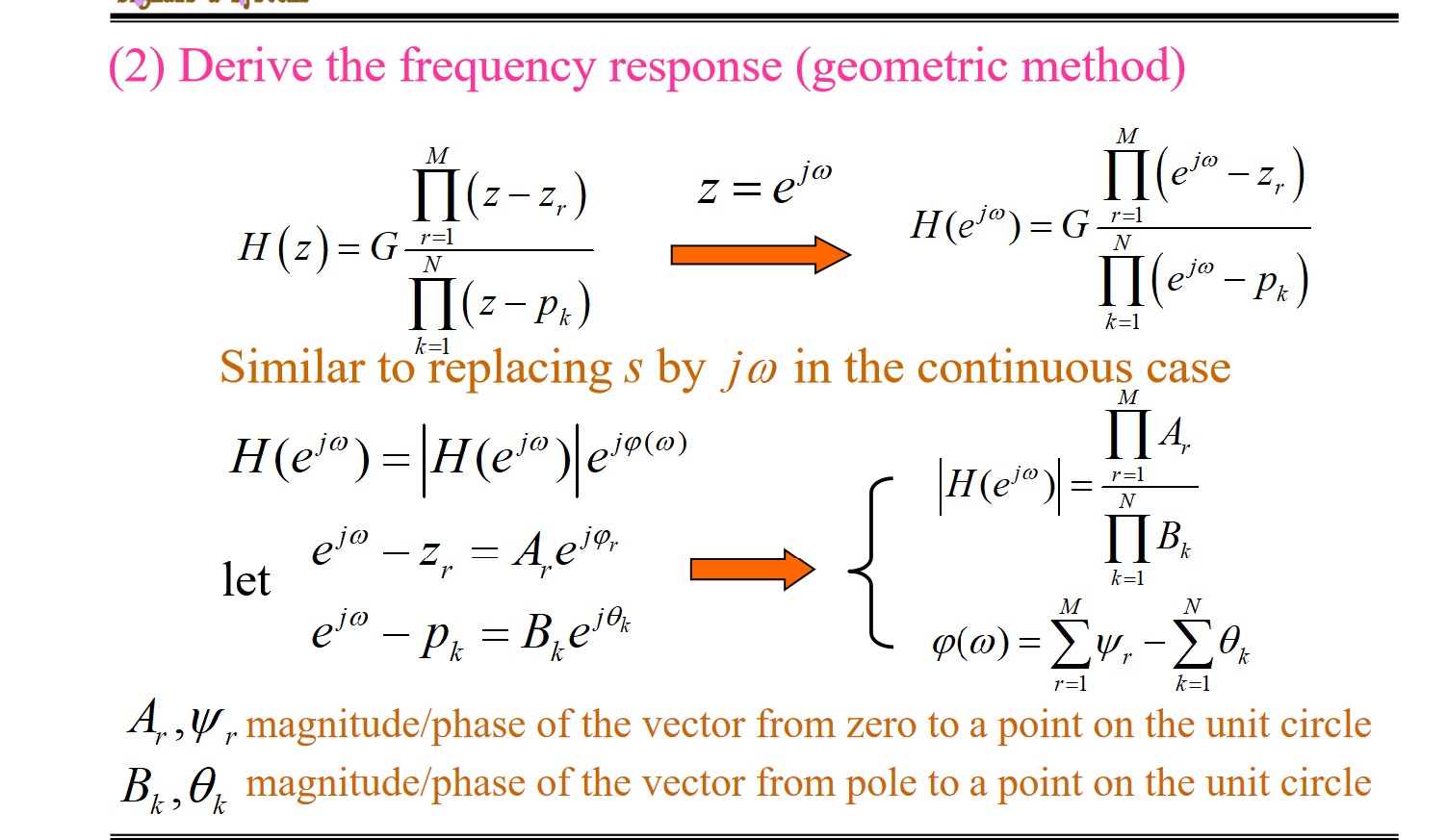
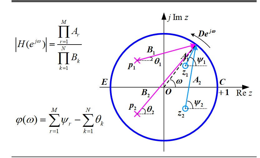
NOTE:
- We can derive the frequency response (function of $\omega$ ) by letting $D$ move along the unit circle once.
- $H(j\omega)$ is periodic. The frequency response from 0 to $\omega_s/2$ can be determined by letting $D$ move along half circle.
- If pole $p_i$ is close to the unit circle, there will be a peak in the frequency response. If zero $z_i$ is close to the unit circle, there will be a notch in the frequency response.
- For statble systems, $p_i$ should be inside the unit circle, while $z_i$ could be inside or outside the unit circle.
- poles and zeros at origin have no influence on amplitude.
Analog and digital Filter
Fundamental Principles
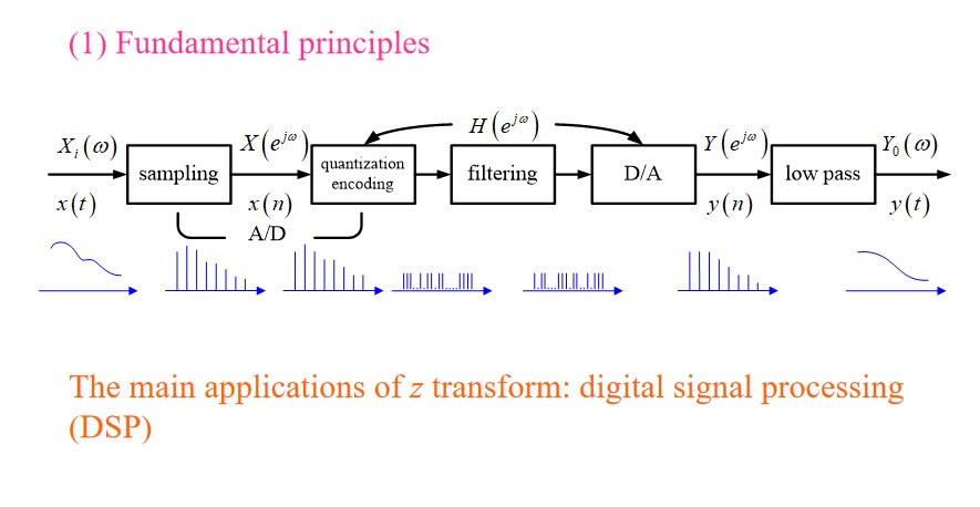
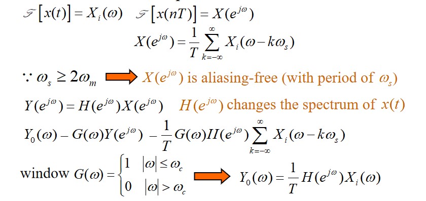
The spectrum of $x(t)$ is strictly inside $\pm \omega_m$ .
We choose the sampling frequency: $\omega_s = \frac{2\pi}{T} \ge 2\omega_m$
Classifications of digital filters
$$ y(n) = \sum_{k=0}^M b_kx(n-k) - \sum_{k=1}^N a_ky(n-k) $$In terms of structure
recursive: $a_k\ne 0$ at least for one $k$
non-recursive: $a_k=0$ , for all $k$
In terms of the characteristics of $h(n)$
Infinite impulse response(IIR): recursive, non-linear phase
Finite impulse response(FIR): non-recursive, linear phase.
IIR filter
Impulse invariance
Based on the s-domain analog filters.
Design method 1: 冲激响应不变法
Replace $\frac{1}{s-s_k}$ with $\frac{1}{1-e^{s_kT}z^{-1}}$ . Then $H_a(s)$ become $H(z)$ .
The relationship between the continuous and discrete filters:
$$ H(z)|_{z = e^{sT}} = \frac{1}{T}\sum_{k=-\infty}^\infty H_a(s + j\frac{2\pi}{T}k) $$The result is just repeat the original filter at sampling frequency, thus it attenuates slower.
NOTE:The digital filter implemented this way has aliasing.
The frequency response of analog filter must be attenuated enough within $\omega_s$ .
This approach can only realize LP and BP filter, but not HP and band-stop one.
method 2: Bilinear transformation emerges to address this problem (you can study it by yourself)
$$ s = \frac{2}{T}\left(\frac{1 - z^{-1}}{1 + z^{-1}}\right)\\ z = \frac{1 + \frac{sT}{2}}{1 - \frac{sT}{2}} $$Bilinear transformation is non-linear transformation.
To implement digital filter, A/D and D/A are required, along with ROM, RAM, ALU, delay units (shift registers), etc.
FIR filter
$$ H(z) = \sum_{k = 0}^{N-1}b_kz^{-k} = \sum_{n=0}^{N-1}h(n)z^{-n} $$Poles are at $z=0$ . $N - 1$ zeros.
FIR filter has linear-phase iff
$$ h(n) = h(N - 1 - n)(\text{evenly symmetric})\\ h(n) = -h(N - 1 - n)(\text{oddly symmetric}) $$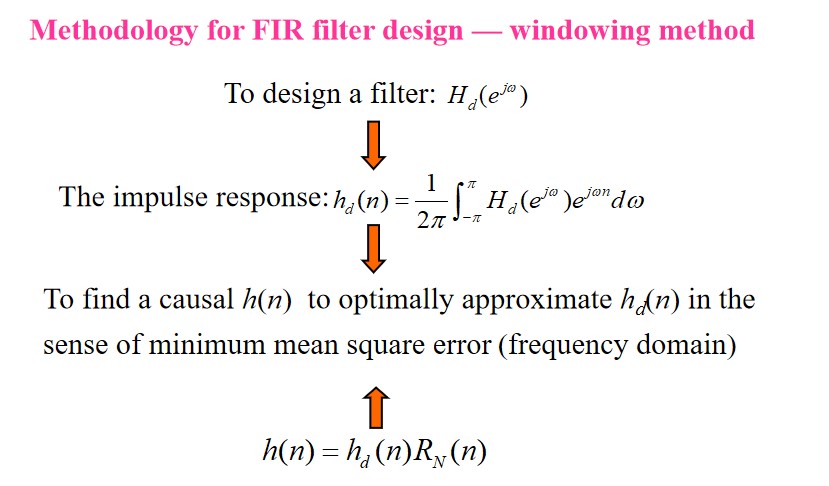
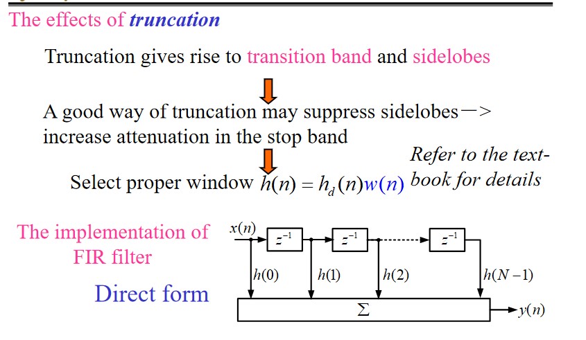
Feedback System: Signal Flow Graphs
Operator and Transfer Operator:
$$ p = \frac{d}{dt}\\ \frac{1}{p} = \int_{-\infty}^t(\cdot)d\tau $$ $$ (C_0p^n + C_1p^{n-1} + \dotsb + C_n)r(t) = (E_0p^m + E_1p^{m - 1} + \dotsb + E_m)e(t)\\ D(p)r(t) = N(p)e(t) $$Rules:
- Common factors can’t be eliminated.
- Be careful when changing the order of operation( $\frac{d}{dt}\int_{-\infty}^tx(\tau)d\tau = x(t)$ , $\int_{-\infty}^t\frac{d}{d\tau}x(\tau)d\tau = x(t) - x(-\infty)$ )
transfer operator:
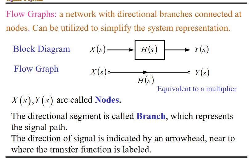
$$ r(t) = \frac{N(t)}{D(t)}e(t) = H(p)e(t) $$Brief introduction to the signal flow graphs(SFG)
Terminnologies in SFG
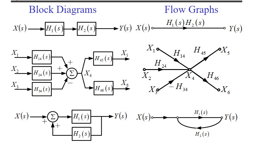
Node, Transfer function, Branch(The branch gain is the transfer function), Source node, Sink node, Mixed node.
Properties of SFG
- Signal only passes through a branch with the direction indicated by the arrowhead.
- Signals of incoming branches are added at a node, and the added signal appears on the all outgoing branches.
- A sink node can be separated from a mixed node.
- For a given system, the SFGs can be different.(equations for a system can be different)
- After the SFG being inversed, the transfer function keeps invariant, but the signals represented by the inner nodes will be different.
Note: Inversion is done by inversing the transfer direction of each branch, and exchanging the source and sink nodes as well.
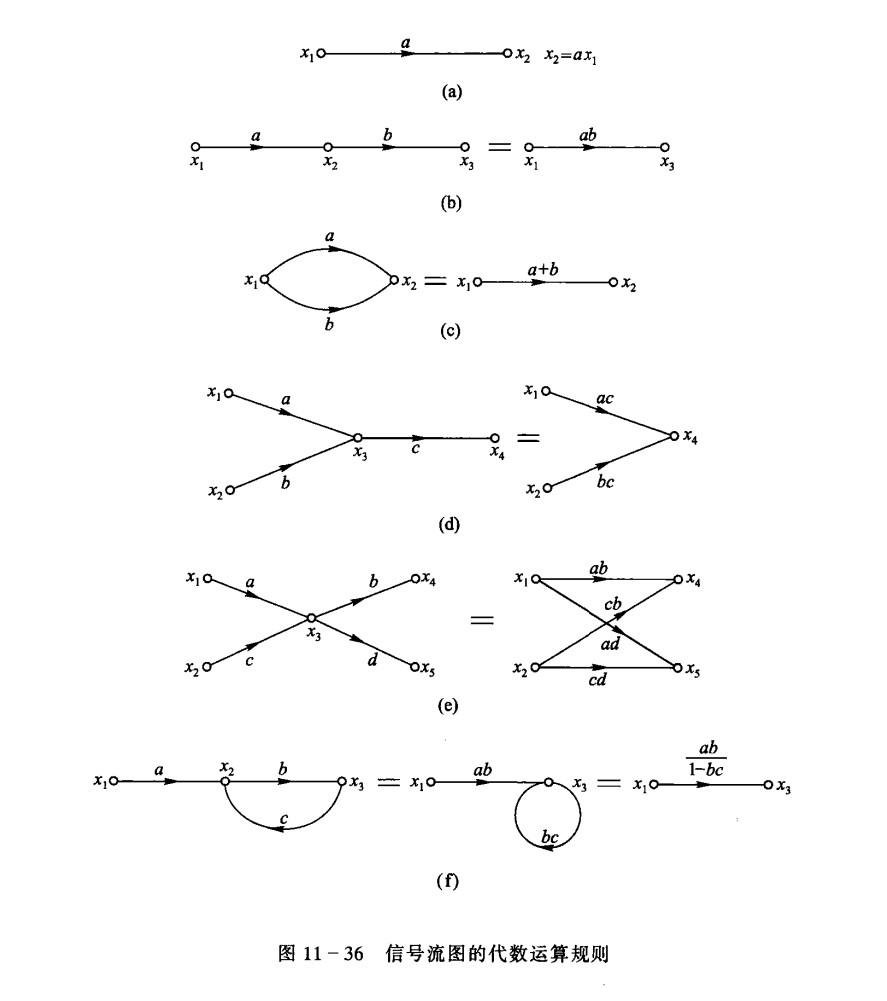
Algebra of SFG
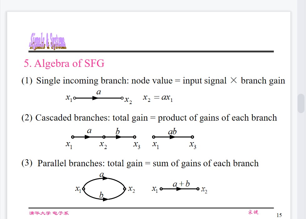
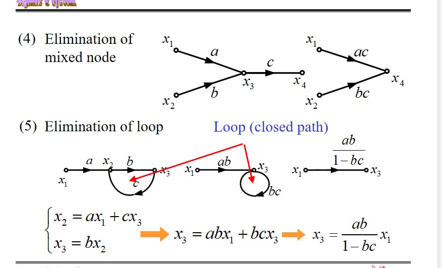
Simplify:
NOTE: The SFG can be simplified using the following steps:
a. Merge the cascaded branches to decrease the number of nodes;
b. Merge the parallel branches to decrease the number of branches;
c. Eliminate all the loops.
Then, the system function can be readily derived.
Mason’s Formula
$$ H = \frac{1}{\Delta} \sum_k g_k\Delta_k $$
State-variable analysis of system
$$ \mathbf {\lambda = A\lambda + Be}\\ \mathbf{r = C\lambda + De} $$Features of the state-variable analytical method
- (1)Provide internal characteristics of the system
- (2) Convenient to represent and analyze the multi-input, multi-output (MIMO) cases
- (3) Easy to be extended to time-variant or nonlinear cases
- (4) Introduce two important concepts: controllability and observability
- (5) Convenient for numerical computation
General form and setup method (CT)
$$ \frac{d}{dt}\mathbf{\lambda}(t)_{k \times 1} = \mathbf{A}_{k \times k}\mathbf{\lambda}(t)_{k \times 1} + \mathbf{B}_{k \times m}\mathbf{e}(t)_{m \times 1}\\ \mathbf{r}(t)_{r \times 1} = \mathbf{C}_{r \times k}\mathbf{\lambda}(t)_{k \times 1} + \mathbf{D}_{r \times m}\mathbf{e}(t)_{m \times 1} $$ $r$ responses, $k$ state variables, $m$ inputs.For time-variant system, $\mathbf{A, B, C, D}$ are fuction of $t$ .
Direct methods:
- observation
- Topological analysis
Used in curcuit analysis.
Indirect methods:
- From block diagram or flow graph
- From input-output equation
- From transfer function
Used in controlled system analysis.
From input-output equation
$$ \frac{r(t)}{e(t)} = \frac{b_0p^k + \dotsb + b_k}{p^k + \dotsb + a_k} $$NOTE : under the zero-state condition, $p$ is equivalent to $s$
$$ H(p) = \frac{b_0 + b_1p^{-1} + \dotsb + b_kp^{-k}}{1 + a_1p^{-1} + \dotsb + a_kp^{-k}} $$The SFG is:
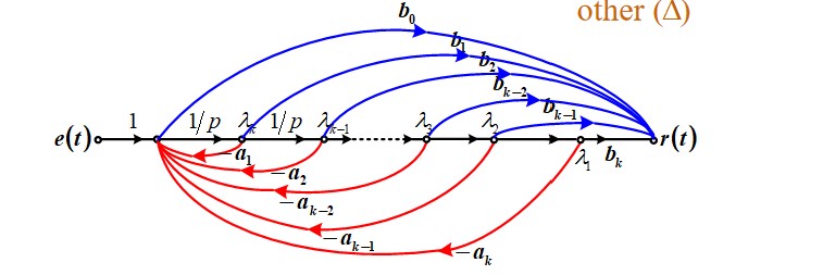
If the order of differential equation on the left side is higher than that on the right side:
$$ b_0 = 0, \mathbf{D} = 0 $$If the derivatives of the excitation on the right side are absent,
$$ \mathbf{C} = [b_k, 0, \dotsb, 0], \mathbf{D} = 0 $$Factorizing Transfer operator
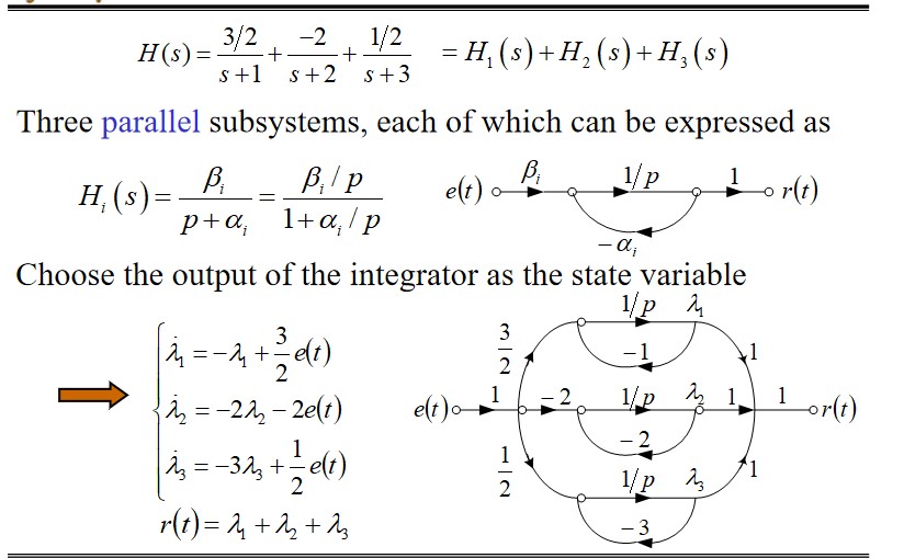
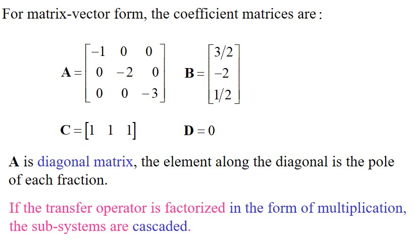
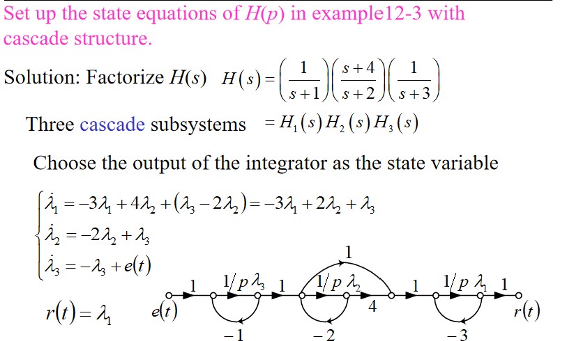
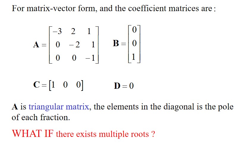
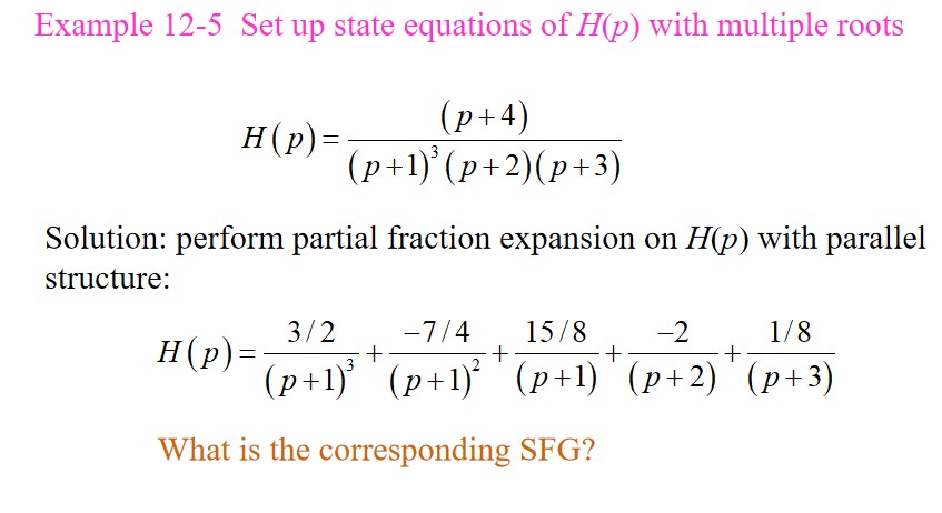
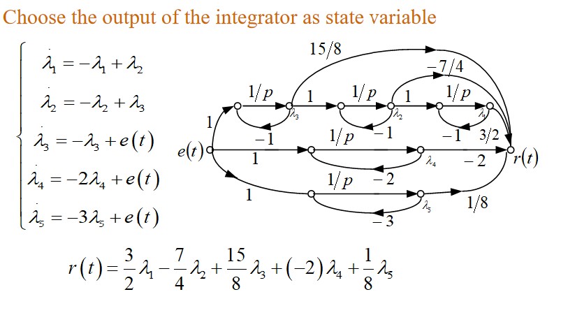
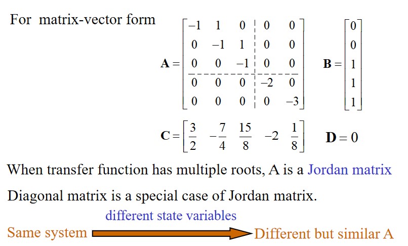
Solving CT system’s state equations
Time domain method using computer.
Transform-domain(Laplace-tranform) method
$$ \frac{d}{dt}\mathbf{}{\lambda}(t) = \mathbf{A\lambda}(t) + \mathbf{Be}(t)\\ \mathbf{r}(t) = \mathbf{C\lambda}(t) + \mathbf{De}(t)\\ \mathbf{\lambda}(0_-) = \begin{bmatrix} \lambda_1(0_-)\\ \lambda_2(0_-)\\ \vdots\\ \lambda_k(0_-)\\ \end{bmatrix} $$ $$ s\mathbf \Lambda(s) - \mathbf{\lambda}(0_-) = \mathbf{A\Lambda}(s) + \mathbf{BE}(s)\\ \mathbf{R}(s) = \mathbf{C\Lambda}(s) + \mathbf{DE}(s) $$ $$ \mathbf{\Lambda}(s) = (s\mathbf {I} - \mathbf{A})^{-1}\mathbf{\lambda}(0_-) + (s\mathbf {I} - \mathbf{A})^{-1}\mathbf{BE}(s)\\ \mathbf R(s) =\mathbf{C} (s\mathbf {I} - \mathbf{A})^{-1}\mathbf{\lambda}(0_-) + (\mathbf C(s\mathbf {I} - \mathbf{A})^{-1}\mathbf{B + D)E}(s) $$Let $\Psi(s) = (s\mathbf I - \mathbf A)^{-1}$ , which is called characteristic matrix.
$$ \mathbf\lambda(t) = \mathcal{L}^{-1}[\Psi(s)\lambda(0_-)] + \mathcal{L}^{-1}[\Psi(s)\mathbf{B}] * e(t)\\ \mathbf r(t) = \mathbf{C}\mathcal{L}^{-1}[\Psi(s)\lambda(0_-)] + \lbrace\mathbf{C}\mathcal{L}^{-1}[\mathbf\Psi(s)\mathbf{B] + D}\delta(t)\rbrace * e(t) $$Time-domain method
$$ e^{\mathbf At} = \sum_{k = 0}^\infty \frac{1}{k!}A^kt^k $$properties
$$ e^{\mathbf At}e^{-\mathbf At} = \mathbf I\\ e^{\mathbf At} = [e^{-\mathbf At}]^{-1}\\ \frac{d}{dt}e^{\mathbf At} = \mathbf Ae^{\mathbf At} = e^{\mathbf At} \mathbf A\\ $$ $$ \frac{d}{dt}\mathbf \lambda(t) = \mathbf A\mathbf \lambda(t) + \mathbf B\mathbf e(t)\\ e^{-\mathbf At}\frac{d}{dt}\mathbf \lambda(t) = e^{-\mathbf At}\mathbf A\mathbf \lambda(t) + e^{-\mathbf At}\mathbf B\mathbf e(t)\\ \frac{d}{dt}e^{-\mathbf At}\mathbf \lambda(t) = e^{-\mathbf At}\mathbf B\mathbf e(t)\\ \lambda(t) = e^{\mathbf At}\mathbf \lambda(0_-) + \int_0^te^{\mathbf A(t - \tau)}\mathbf B\mathbf e(\tau)d\tau\\ =e^{\mathbf At}\lambda(0_-) + e^{\mathbf At} \mathbf B * \mathbf e(t) $$output
$$ \mathbf r(t) = \mathbf C e^{\mathbf At}\mathbf \lambda(0_-) + \mathbf C e^{\mathbf At} \mathbf B * \mathbf e(t) + \mathbf D\mathbf e(t)\\ = \mathbf C e^{\mathbf At}\mathbf \lambda(0_-) + [\mathbf C e^{\mathbf At} \mathbf B + \mathbf D\delta(t)] * \mathbf e(t) $$Correspond to LT:
$$ \mathcal{L}[e^{\mathbf At}] = (s\mathbf I - \mathbf A)^{-1} $$Derive System Functions
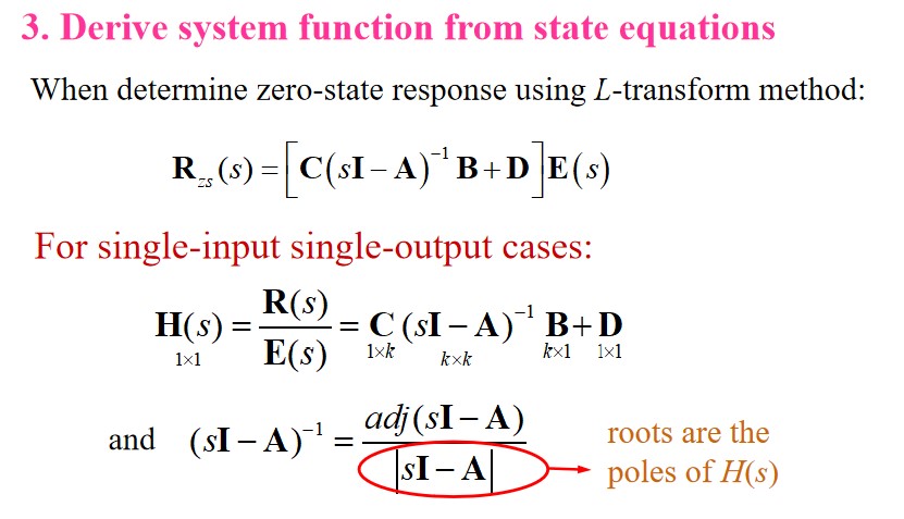
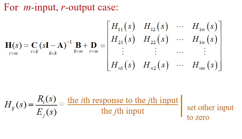
That for DT system
State equation setup
$$ \begin{align*} \mathrm\lambda(n + 1) &= \mathbf A\mathrm\lambda(n) + \mathbf B\mathrm x(n)\\ \mathrm y(n) &= \mathbf C\mathrm\lambda(n) + \mathbf D\mathrm x(n) \end{align*} $$Solving:
$$ \lambda(n) = \underbrace{A^n\lambda(0)u(n)}_{\text{Zero Input}} + \underbrace{\left[\sum_{i=0}^{n-1}A^{n-1-i}Bx(i)\right]u(n-1)}_{\text{Zero State}}\\ y(n) = \underbrace{CA^n\lambda(0)u(n)}_{\text{Zero Input}} + \underbrace{\left[\sum_{i=0}^{n-1}CA^{n-1-i}Bx(i)\right]u(n-1) + Dx(n)u(n)}_{\text{Zero State}} $$The Impulse response is:
$$ h(n) = CA^{n-1}Bu(n-1) + D\delta(n) $$Calculate $A^n$ : Cayley-Hamilton Theorem
ZT Solution
$$ \begin{align*} z\mathrm\Lambda(z) - z\lambda(0) &= \mathbf A\mathrm\Lambda(z) + \mathbf B\mathrm X(z)\\ \mathrm Y(z) &= \mathbf C\mathrm\Lambda(z) + \mathbf D\mathrm X(z) \end{align*} $$ $$ \mathrm \Lambda(z) = (z\mathbf I - \mathbf A)^{-1}\lambda(0) + (z\mathbf I - \mathbf A)^{-1}\mathbf B\mathrm X(z)\\ \mathrm Y(z) = \mathbf C(z\mathbf I - \mathbf A)^{-1}\lambda(0) + \left[\mathbf C(z\mathbf I - \mathbf A)^{-1}\mathbf B + \mathbf D\right]\mathrm X(z) $$then
$$ \lambda(n) = \mathcal{Z}^{-1}\left[(z\mathbf I - \mathbf A)^{-1}z\right]\lambda(0) + \mathcal{Z}^{-1}\left[(z\mathbf I - \mathbf A)^{-1}\mathbf B\right] * \mathcal{Z}^{-1}\left[\mathrm X(z)\right]\\ y(n) = \mathcal{Z}^{-1}\left[\mathbf C(z\mathbf I - \mathbf A)^{-1}z\right]\lambda(0) + \mathcal{Z}^{-1}\left[\mathbf C(z\mathbf I - \mathbf A)^{-1}\mathbf B + \mathbf D\right] * \mathcal{Z}^{-1}\left[\mathrm X(z)\right] $$Comparing this with CT solution, we find
$$ A^n = \mathcal{Z}^{-1}\left[(\mathbf I - z^{-1}\mathbf A)^{-1}\right]\\ $$ $$ H(z) = C(\mathbf I - z^{-1}\mathbf A)^{-1}\mathbf B + D $$Linear Transform on state vectors
$$ \mathbf{\gamma} = \mathbf P\mathbf \lambda $$The equations become:
$$ \frac{d}{dt}\gamma(t) =\mathbf{PAP}^{-1}\mathbf \gamma(t) + \mathbf{PB}e(t)\\ \mathbf y(t) = \mathbf {CP}^{-1}\gamma(t) + \mathbf D\mathbf e(t) $$Similarity transform doesn’t change the eigenvalues.
Transform function matrix keeps invariant under linear transformation.
We can diagonalize the matrix A.
Calculate eigenvalues $\alpha$ -> calulate eigenvectors $\xi$ -> $\mathbf P^{-1} = [\xi_i]$ , $\hat A = \text{diag}(\alpha_i)$
Controllable & Observable
Controllable is
$$ \text{rank} [A\ AB\ \dots\ A^{k-1}B] \text{ is full} $$Uncontrollabilty is the input can’t change the response.
Obeservability is
$$ \text{rank} \begin{bmatrix} C\\ CA\\ \vdots\\ CA^{k-1} \end{bmatrix} \text{ is full} $$Unobserverbility is the response is not affected by the input.
After the diagonalization of A:
B doesnt contain zero $\Leftrightarrow$ completely controllable. Otherwise, the 0s is coresponding to the uncontrollable state variables.
C doesnt contain zero $\Leftrightarrow$ completely observable. Otherwise, the 0s is coresponding to the unobservable state variables.
In fact:
$$ H(s) = C(s\mathbf I - \mathbf A)^{-1}\mathbf B + D \stackrel{D = 0}{=} \sum_{i=1}^n \frac{C_iB_i}{s - \alpha_i} $$The $H(s)$ only contains the controllable and observable state variables. So the state and output equations contains more information than the $H(s)$ .
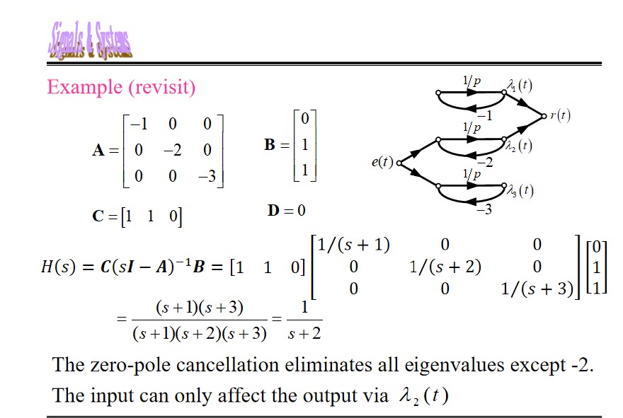
CDMA
Use a set of orthogonal codes to support multiple users by orthorgonal multiplexing.
Example
Assume K users need to connect with the base station simultaneously for CDMA system.
- Design a set of orthogonal codes
- Design on the transmitter
- Design on the receiver
An example of Code 4:
$$ \begin{align*} \mathbf c_1 &= [1\ 1\ 1\ 1\ -1\ -1\ -1\ -1]\\ \mathbf c_2 &= [1\ 1\ -1\ -1\ 1\ 1\ -1\ -1]\\ \mathbf c_3 &= [1\ -1\ 1\ -1\ 1\ -1\ 1\ -1]\\ \mathbf c_4 &= [1\ -1\ -1\ 1\ 1\ -1\ -1\ 1] \end{align*} $$ $$ R_{x, y}(j) = \begin{cases} \sum_{k = 0}^{N - 1 - j} x(k)y(k + j), &0 \le j \le N - 1\\ \sum_{k = 0}^{N - 1 + j} x(k - j)y(k), &-N + 1 \le j \le 0\\ 0, & |j| \ge N \end{cases} $$Must satisfy:
$$ R_{k, i} \begin{cases} =T, &k = i, \tau=0\\ \ll T, &k \ne i \text{ or } \tau \ne 0 \end{cases} $$second:
(1) frequency shifting: $d_k(t)\cos(\omega t)$
(2) spreading: $s_k(t) = d_k(t)c_k(t)\cos(\omega t)$
third: coherent detection/de-spreading
Core:
- Orthogonal code design(signal design)
- Code capturing and tracking(signal processing and system design)
- Multi-use detection and channel estimation(singal processing and system design)
Code design
requirements:
- sharp auto-correlation curve
- zero cross-correlation
- largest possible orthogonal code set
- highest possible complexity for security performance
Commonly used codes:
- Walsh code
- PN sequence
- GOLD codes
- sliding window capturing
- multiple correlators to detect phase match
The period of address code is much shorter than the period of data code: $T_c < T_d$ , so the modulated signal is much wider in FD, whose spectrum is called spread spectrum.