Learning
Linear Classification
Logistic Regression
Useful for classification problems.
Cross-Entropy Loss
$$ \ell(h(\boldsymbol{x}_{i}),y_{i})=\begin{cases}-\log[\sigma(\boldsymbol{w}^{T}\boldsymbol{x}_{i})]&\quad y_{i}=1\\-\log[1-\sigma(\boldsymbol{w}^{T}\boldsymbol{x}_{i})]&\quad y_{i}=0\end{cases} $$With regularization:
$$ \hat{\epsilon}(w)=-\sum_{i=1}^n\{y_i\log\sigma(h_w(x))+(1-y_i)\log[1-\sigma(h_w(x))]+\lambda\sum_{j=1}^dw_j^2 $$How to deal with multiclass problems?
Softmax Regression
Normalizes multiple outputs in a probability vector.
$$ p(y=i|x)=\frac{\exp(w_i^Tx)}{\sum_{r=1}^C\exp(w_r^Tx)} $$Cross-Entropy Loss
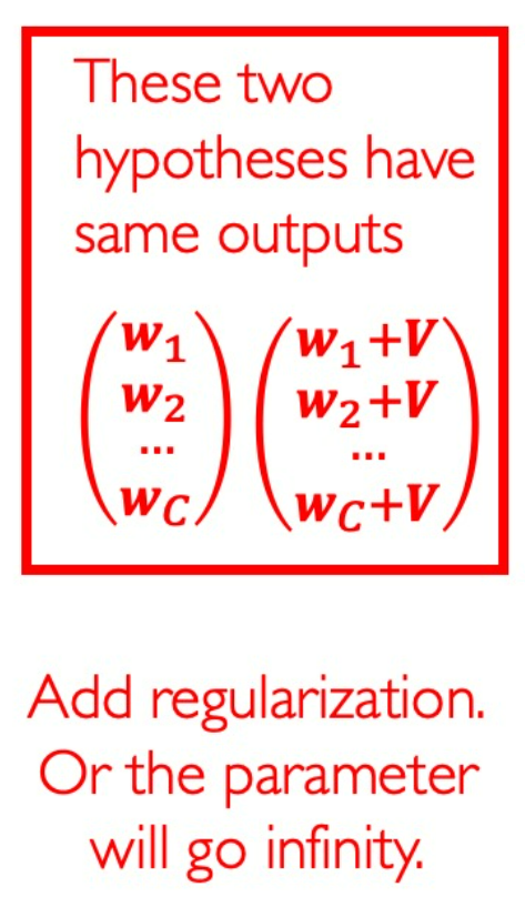
$$ \ell(h(x_i),y_i)=\begin{cases}-\log\left[\frac{\exp(\boldsymbol{w}_1^T\boldsymbol{x})}{\sum_{r=1}^C\exp(\boldsymbol{w}_r^T\boldsymbol{x})}\right]&y_i=1\\-\log\left[\frac{\exp(\boldsymbol{w}_2^T\boldsymbol{x})}{\sum_{r=1}^C\exp(\boldsymbol{w}_r^T\boldsymbol{x})}\right]&y_i=2\\\vdots\\-\log\left[\frac{\exp(\boldsymbol{w}_c^T\boldsymbol{x})}{\sum_{r=1}^C\exp(\boldsymbol{w}_r^T\boldsymbol{x})}\right]&y_i=C\end{cases} $$This loss is convex. But there are many solutions that result in same outputs, so the regularizaton is indispensible to prevent divergence.
Support Vector Machine (SVM)
Soft-SVM (Hinge Loss)
$$ \min_{w,b,\xi}\frac{1}{2}\|w\|_{2}^{2}+\frac{C}{n}\sum_{i=1}^{n}\xi_{i}\\\mathrm{s.t.~}y_i(\boldsymbol{w}\cdot\boldsymbol{x}_i+b)\geq1-\xi_i\\\xi_i\geq0,1\leq i\leq n $$Define Hinge Loss
$$ \ell(f(x),y)=\max\{0,1-yf(x)\} $$For the linear hypothesis:
$$ \ell(f(x),y)=\max\{0,1-y(w\cdot x+b)\} $$Theorem: Soft-SVM is equivalent to a Regularized Rise Minimization:
$$ \min_{w,b}\frac12\|w\|_2^2+\frac Cn\sum_{i=1}^n\max\{0,1-y_i(w\cdot x_i+b)\} $$这意味着SVM的“最大化”边界距离项本质上是一个正则化项。
Kernel Soft-SVM
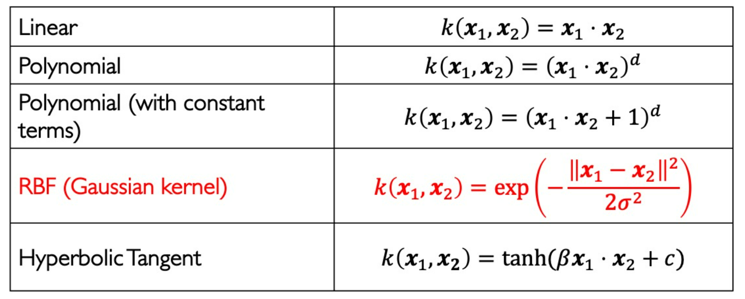
Basis function $\Phi(x)$ can often replaced by kernal function $k(x_1, x_2)$ .
Polynomial Kernel: efficient computation: $O(d)$
Construct new kernel function from exist kernel functions:
$$ k^{\prime}(x_{1},x_{2})=k_{1}\otimes k_{2}(x_{1},x_{2})=k_{1} (x_{1},x_{2})k_{2}(x_{1},x_{2}) $$For any function $g: \mathcal X \rightarrow \R$
$$ k^\prime(x_1,x_2)=g(x_1)k_1(x_1,x_2)g(x_2) $$Apply Representer theorem:
$$ \min_\alpha\frac12\alpha^TK\alpha+\frac Cn\sum_{i=1}^n\max\left\{0,1-y_i\sum_{j=1}^n\alpha_jk(x_i,x_j)\right\} $$- $\alpha_j$ is the weight of each reference point $\color{red}{x_j}$ to the prediction of $\color{red}{x_i}$ .
- lt is actually a Primal Form with kernel functions.
Decision Tree
Criterion:
- More balance
- More pure
Misclassification error (not used very frequently):
$$ \mathrm{Err}(\mathcal{D})=1-\max_{1\leq k\leq K}\left(\frac{|\mathcal{C}_k|}{|\mathcal{D}|}\right) $$Use Entropy to measure purity:
$$ H(\mathcal{D})=-\sum_{k=1}^K\frac{|\mathcal{C}_k|}{|\mathcal{D}|}\mathrm{log}\frac{|\mathcal{C}_k|}{|\mathcal{D}|} $$Gini Index:
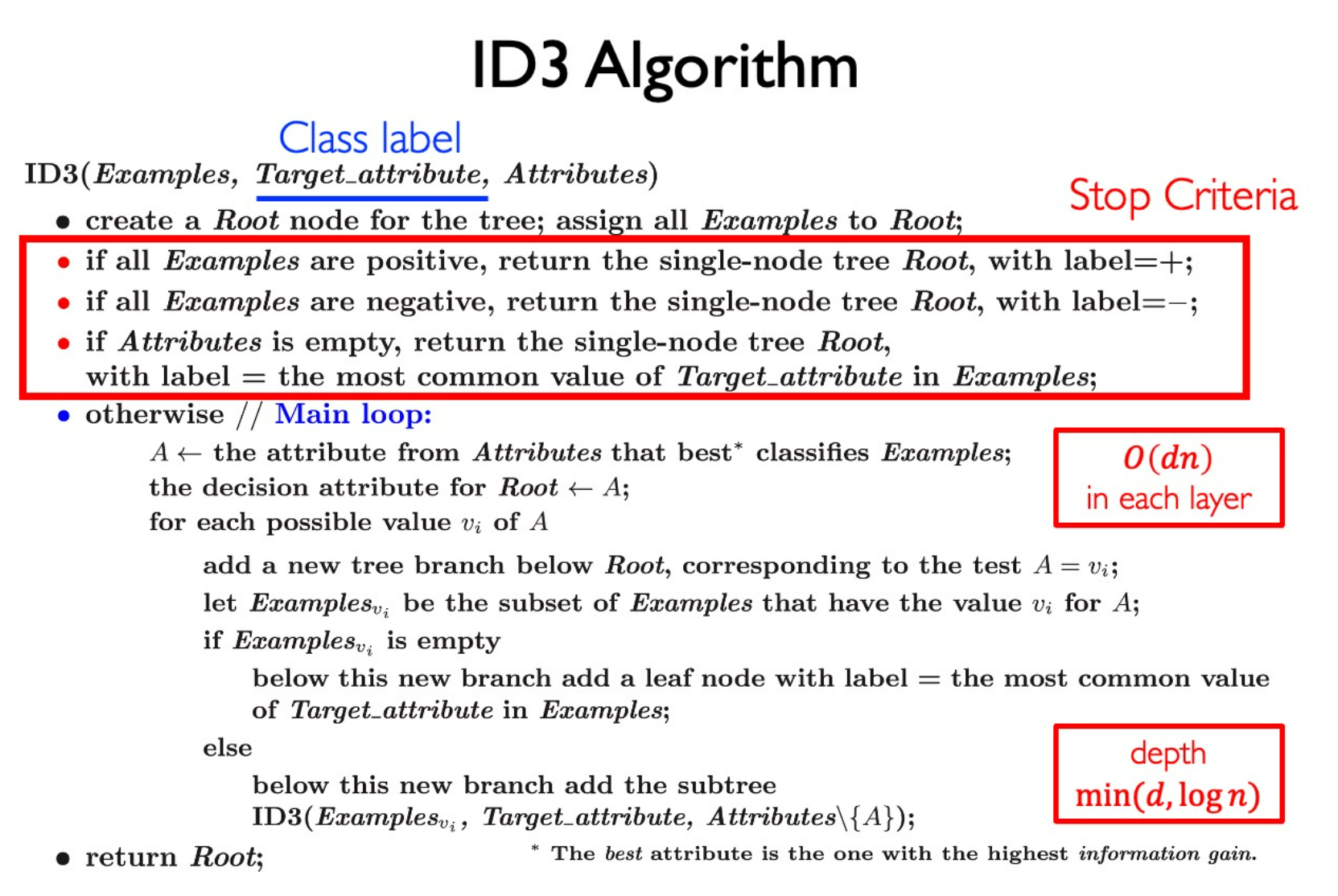
$$ \mathrm{Gini}(\mathcal{D})=1-\sum_{k=1}^K\left(\frac{|\mathcal{C}_k|}{|\mathcal{D}|}\right)^2 $$ID3 Algorithm
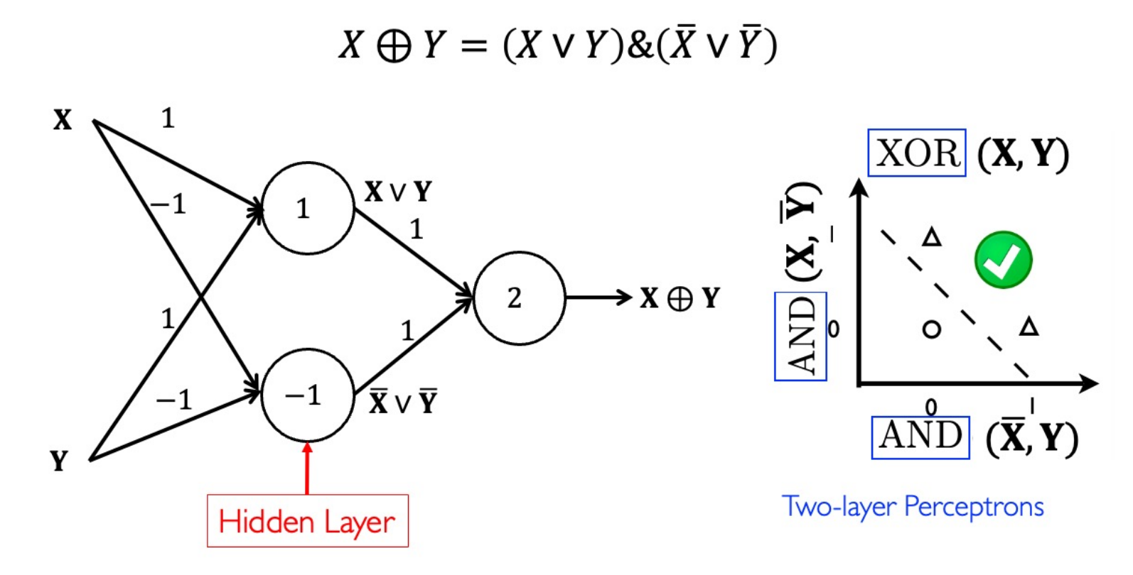
Multiplayer Perceptrons (MLP)
MLP for XOR
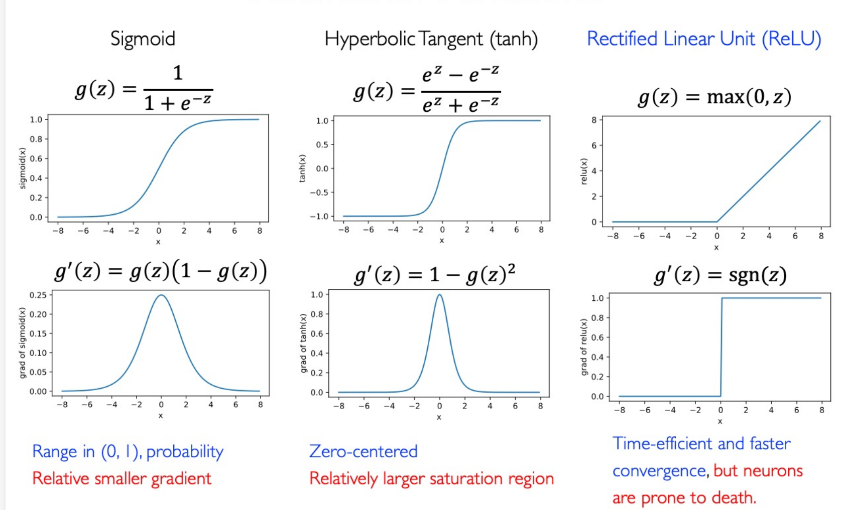
Activation
Loss Functions
Entropy
$$ H(q)=-\sum_{j=1}^kq_j\log q_j $$Relative-entropy
$$ \mathrm{KL}(q||p)=-\sum_{j=1}^kq_j\log p_j-H(q) $$Cross-entropy
$$ H(q,p)=-\sum_{j=1}^kq_j\log p_j $$Relationship:
$$ \boxed{H(q,p)=\mathrm{KL}(q||p)+H(q)} $$Softmax in the output layer
$$ \widehat{\boldsymbol{y}}=\boldsymbol{a}^{(n_l)}=f_\theta\big(\boldsymbol{x}^{(i)}\big)=\begin{bmatrix}p\big(\boldsymbol{y}^{(i)}=1\big|\boldsymbol{x}^{(i)};\boldsymbol{\theta}\big)\\p\big(\boldsymbol{y}^{(i)}=2\big|\boldsymbol{x}^{(i)};\boldsymbol{\theta}\big)\\\vdots\\p\big(\boldsymbol{y}^{(i)}=k\big|\boldsymbol{x}^{(i)};\boldsymbol{\theta}\big)\end{bmatrix}=\frac{1}{\sum_{j=1}^{k}\exp(z_{j}^{(n_{l})})}\begin{bmatrix}\exp(z_{1}^{(n_{l})})\\\exp(z_{2}^{(n_{l})})\\\vdots\\\exp(z_{k}^{(n_{l})})\end{bmatrix} $$Cross-entropy loss:
$$ J(y,\widehat{y})=-\sum_{j=1}^ky_j\log\widehat{y}_j $$Cost function:
$$ \min J(\theta)=-\frac1m\sum_{i=1}^m\left[\sum_{j=1}^k\mathbf{1}\{y^{(i)}=j\}\mathrm{log}\frac{\exp(\mathbf{z}_j^{(n_\iota)})}{\sum_{j^{\prime}=1}^k\exp(\mathbf{z}_{j^{\prime}}^{(n_\iota)})}\right] $$Gradient-Based Training
$$ \arg\min_\theta O(\mathcal{D};\theta)=\sum_{i=1}^mL\left(y_i,f(x_i);\theta\right)+\Omega(\theta) $$Forward Propagation: to compute activations & objective $J(\theta)$
Backward Propagation: Update paramters in all layers
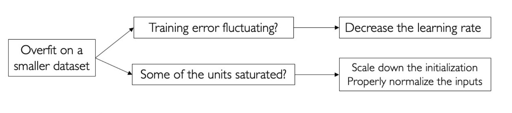
Learning Rate decay
Exponential decay strategy:
$$ \eta = \eta_0e^{kt} $$1/t decay strategy:
$$ \eta = \eta_0/(1+kt) $$Weight Decay
L2 regularization:
$$ \Omega(\theta)=\frac\lambda2\sum_{l=1}^{n_l-1}\sum_{i=1}^{s_l}\sum_{j=1}^{s_{l+1}}(\theta_{ji}^{(l)})^2\\\frac\partial{\partial\theta^{(l)}}\Omega(\theta)=\lambda\theta^{(l)} $$L1:
$$ \Omega(\theta)=\lambda\sum_{l=1}^{n_{l}-1}\sum_{i=1}^{s_{l}}\sum_{j=1}^{s_{l+1}}|\theta_{ji}^{(l)}|\\\frac{\partial}{\partial\theta^{(l)}}\Omega(\theta)_{ji}=\lambda(1_{\theta_{ji}^{(l)}>0}-1_{\theta_{ji}^{(l)}<0}) $$一般不调。
Weight Initialization
Xavier initialization
(Linear activations)
$$ \mathrm{Var}(w)=1/n_{\mathrm{in}} $$避免梯度爆炸或者消失;
He initialization
(ReLU activations)
$$ \mathrm{Var}(w)=2/n_{\mathrm{in}} $$因为 ReLU 删除了一半的信息。
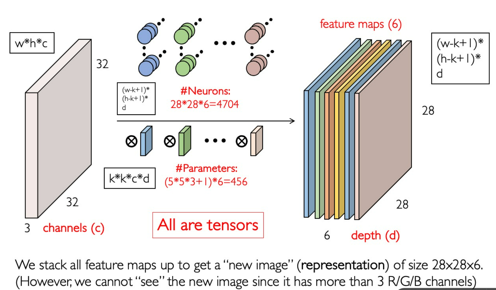
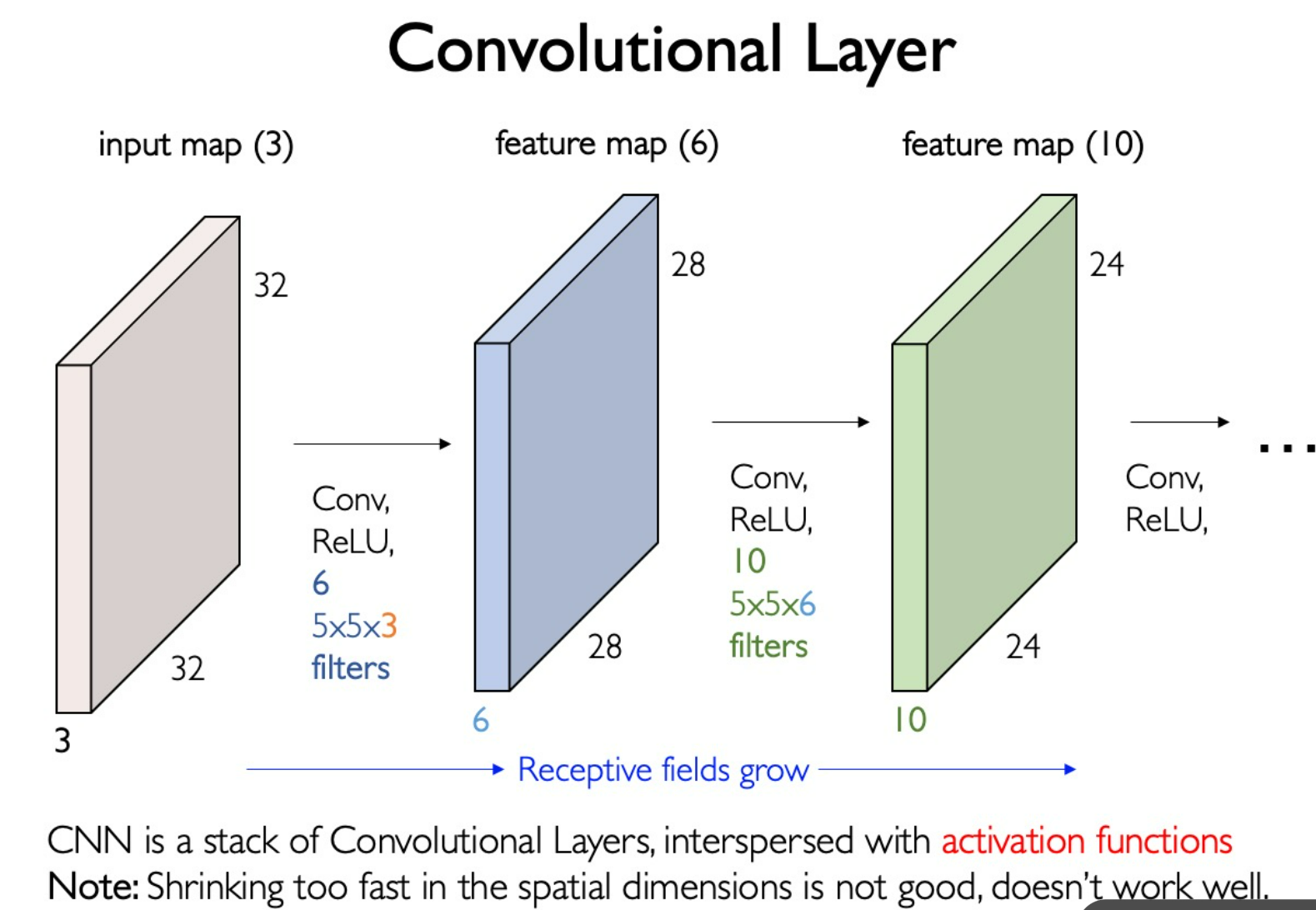
Convolutional Neural Network (CNN)
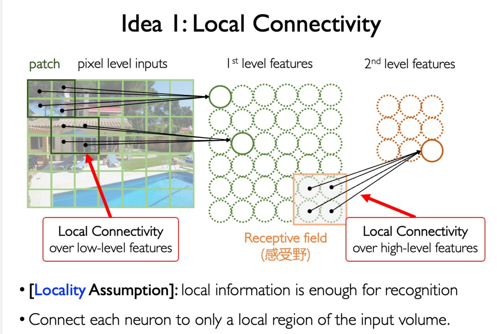
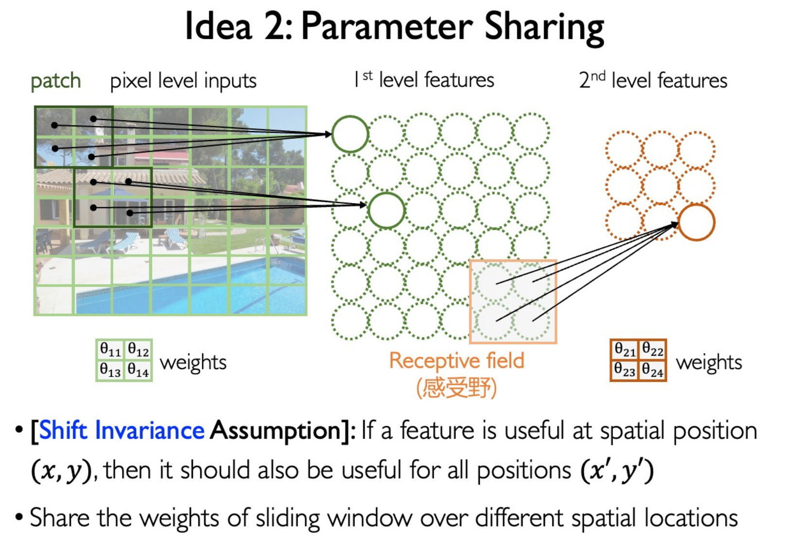
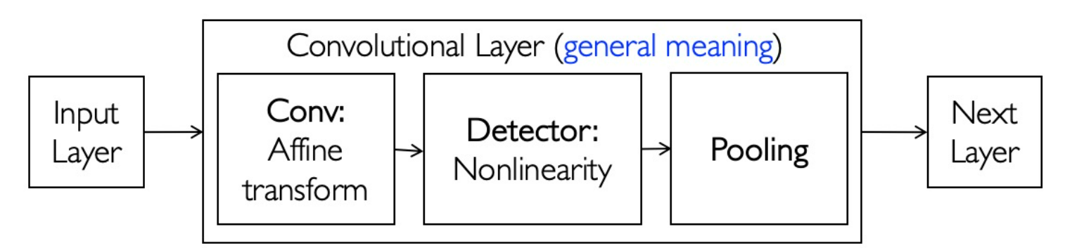
Convoluion Kernel
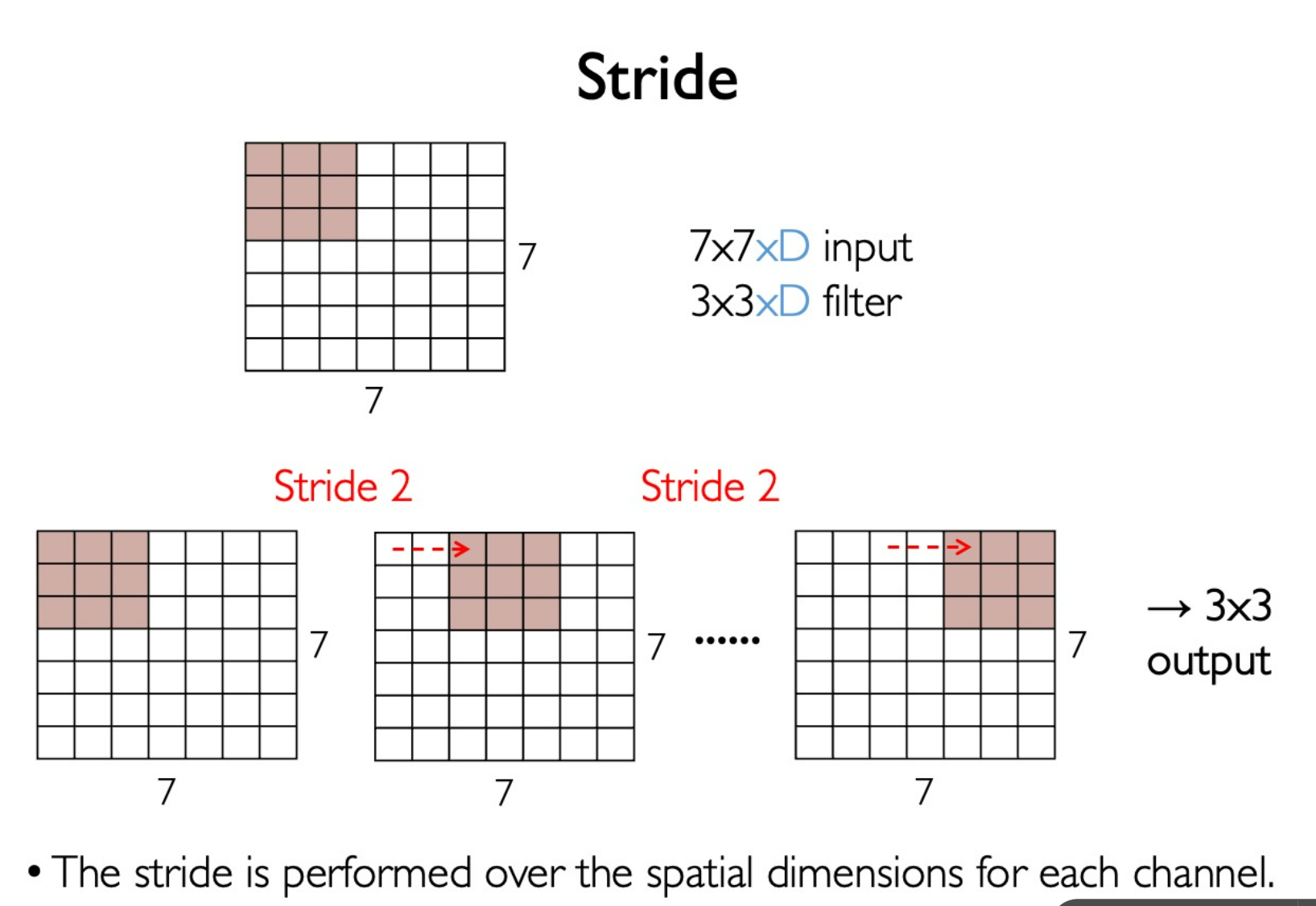
Stride
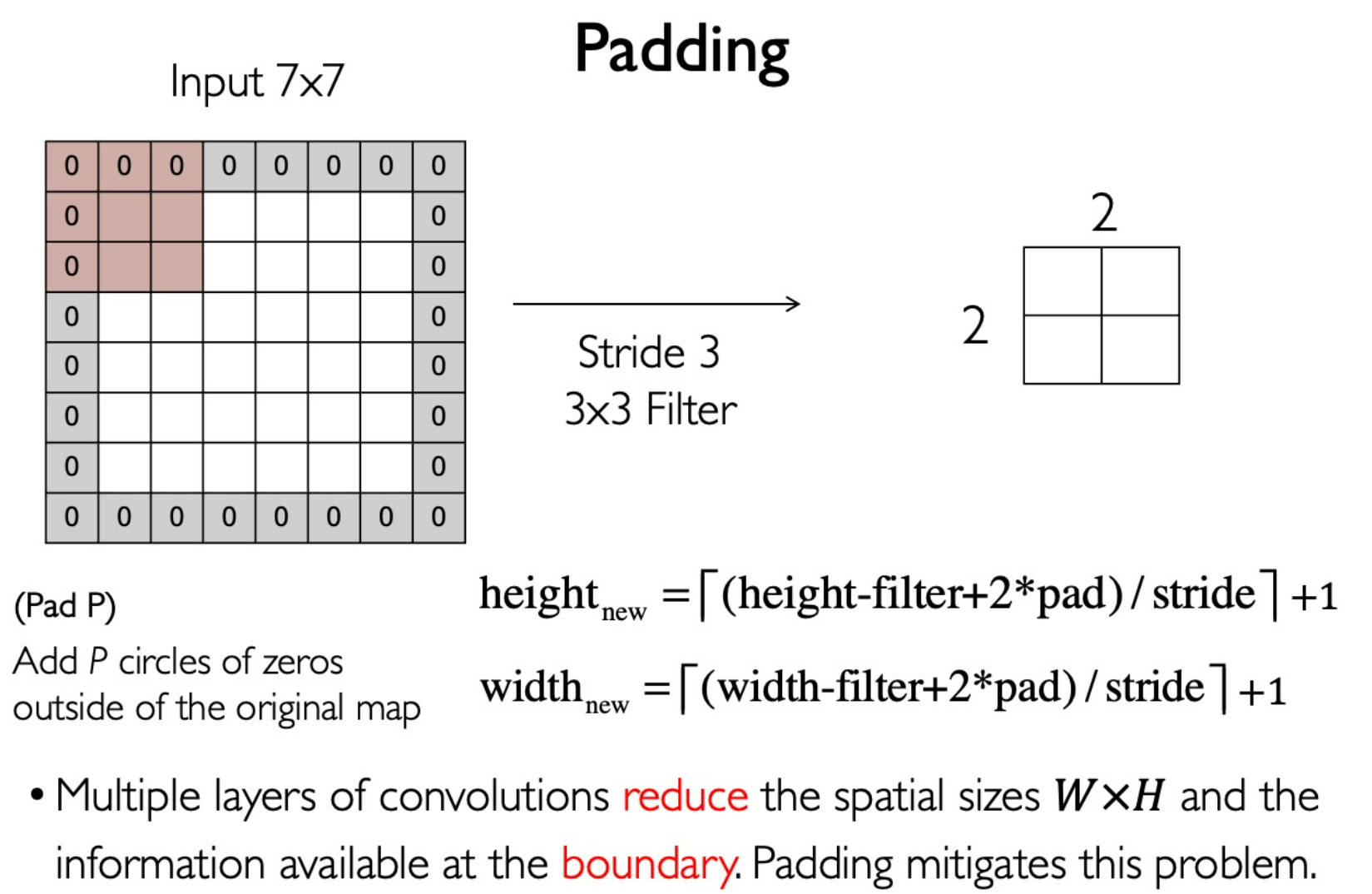
Padding
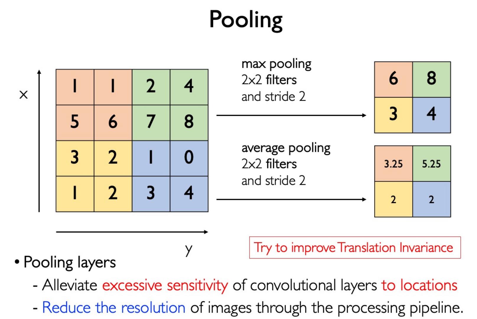
Pooling
Batch Normalization
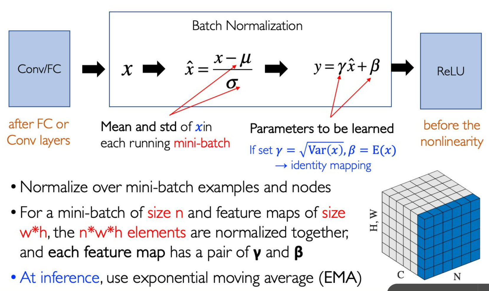
在 N 张图像的对应通道做归一化。
可以增强训练的稳定性,使得学习率可以设大一点而仍然保证收敛。
- 数据集成
- 参数集成
- 模型集成
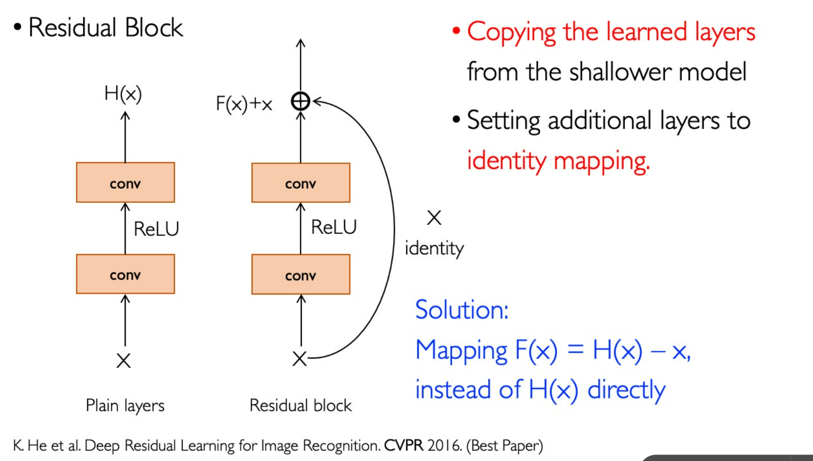
ResNet
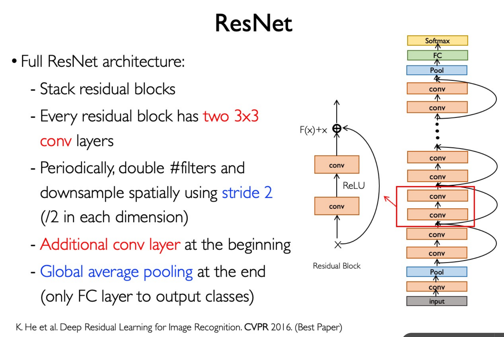
最后一层 Global Average Pooling:7*7*2048 -> 1* 1 * 2048
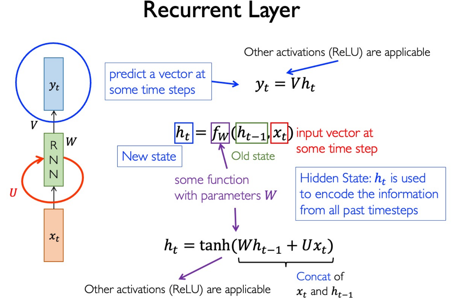
Recurrent Neural Network (RNN)
Idea for Sequence Modeling
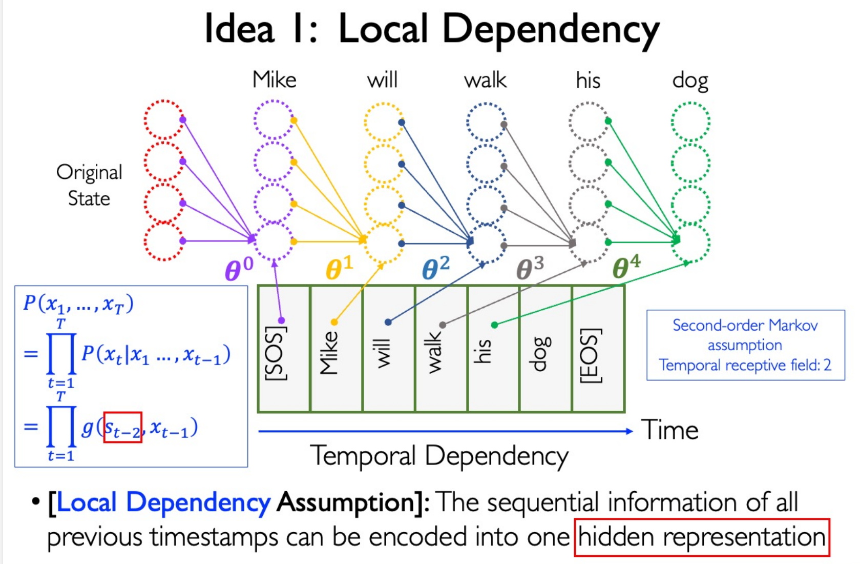
Local Dependency
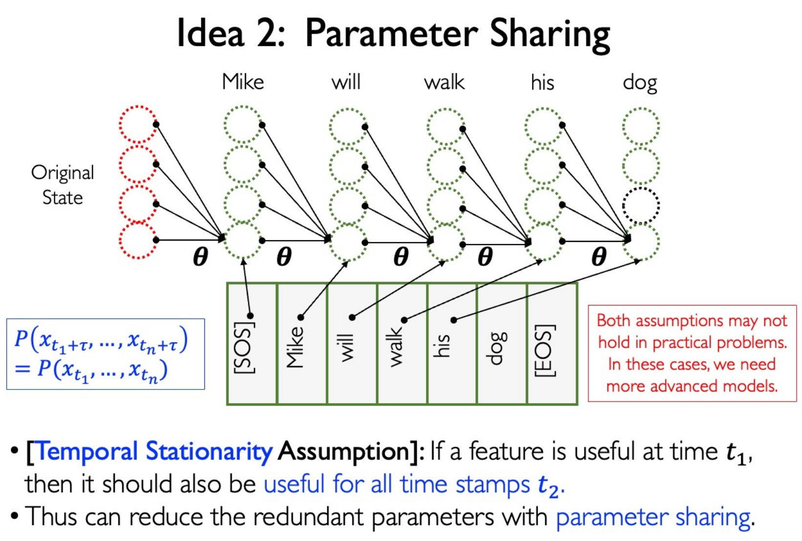
Parameter Sharing
RNN
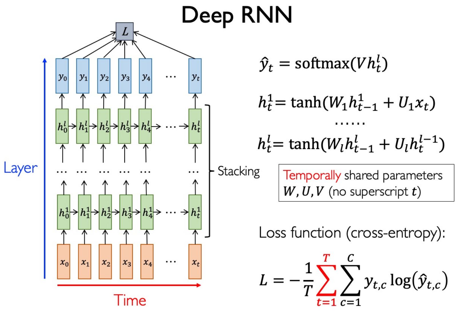
Go deeper
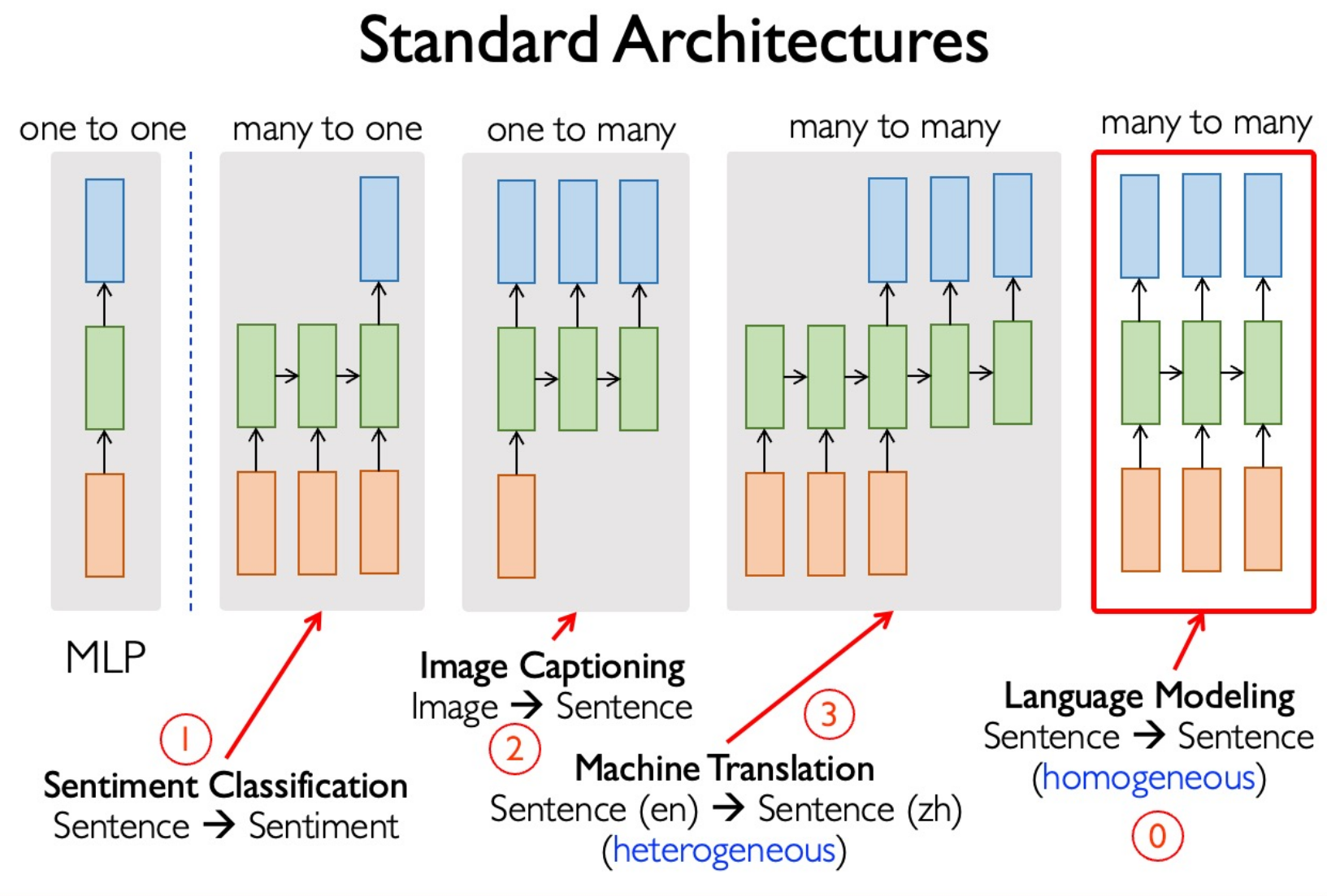
Standard Architectures
- RNNs can represent unbounded temporal dependencies
- RNNs encode histories of words into a fixed size hidden vector
- Parameter size does not grow with the length of dependencies
- RNNs are hard to learn long range dependencies present in data
LSTM
Multihead, shared bottom.
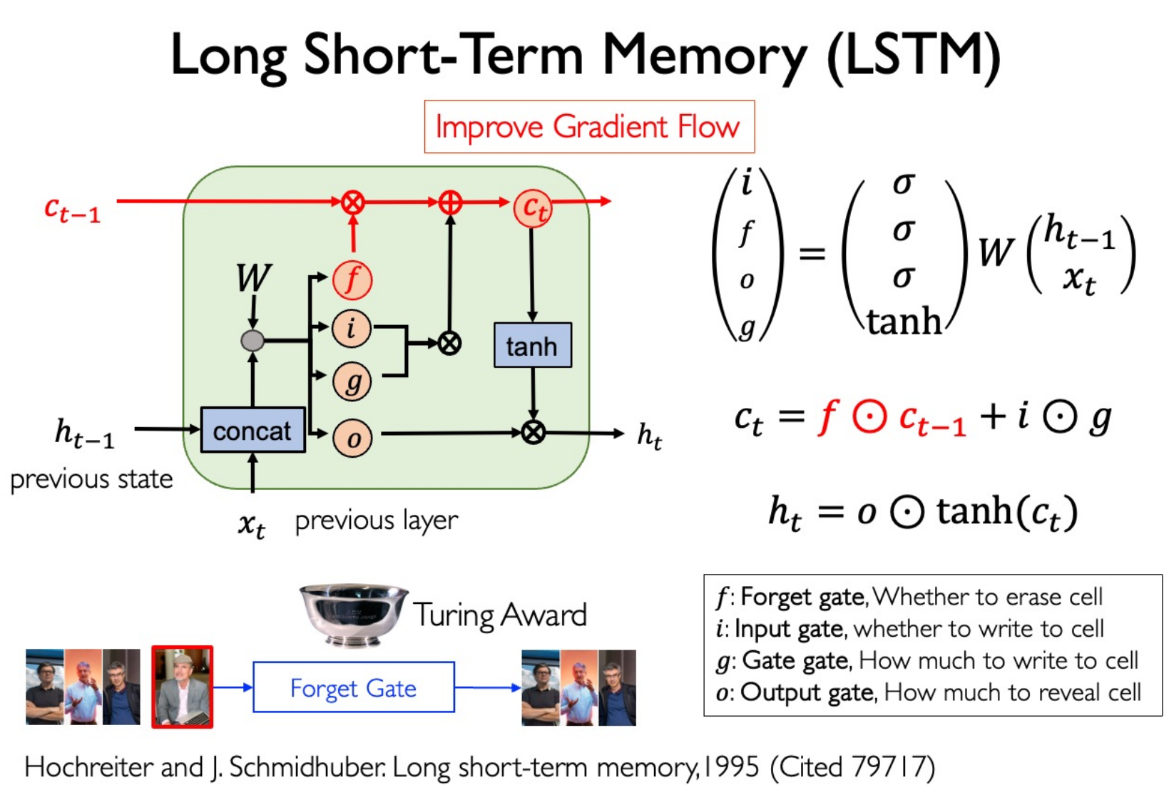
Gradient flow highway: remember history very well.
NIPS 2015 Highway Network.
Training Strategies
Shift in Training & Inference
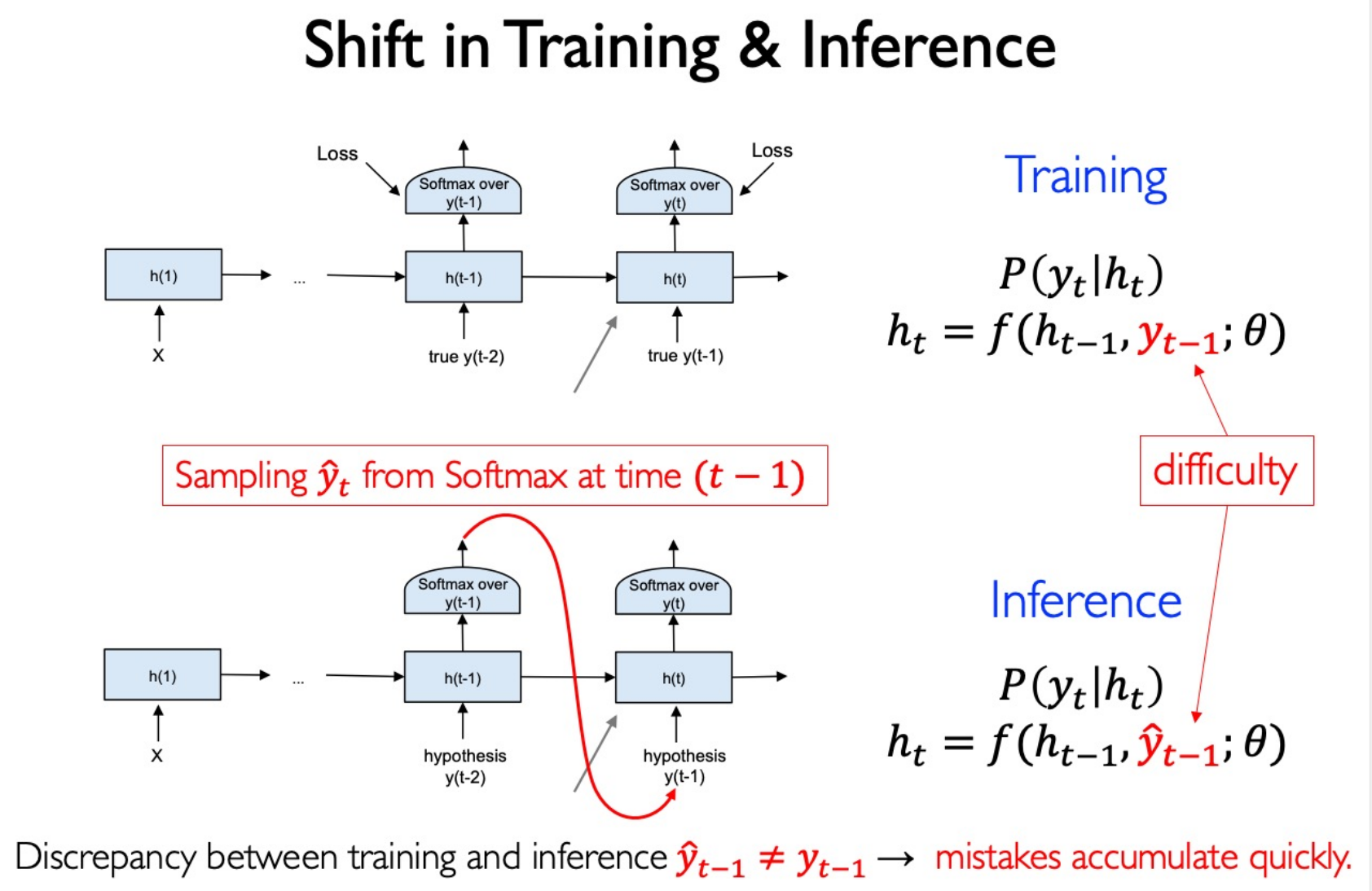
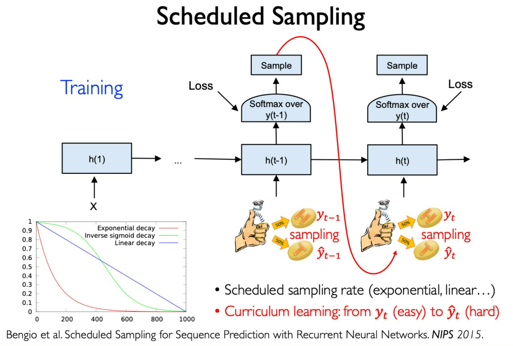
Use Scheduled Sampling to solve this
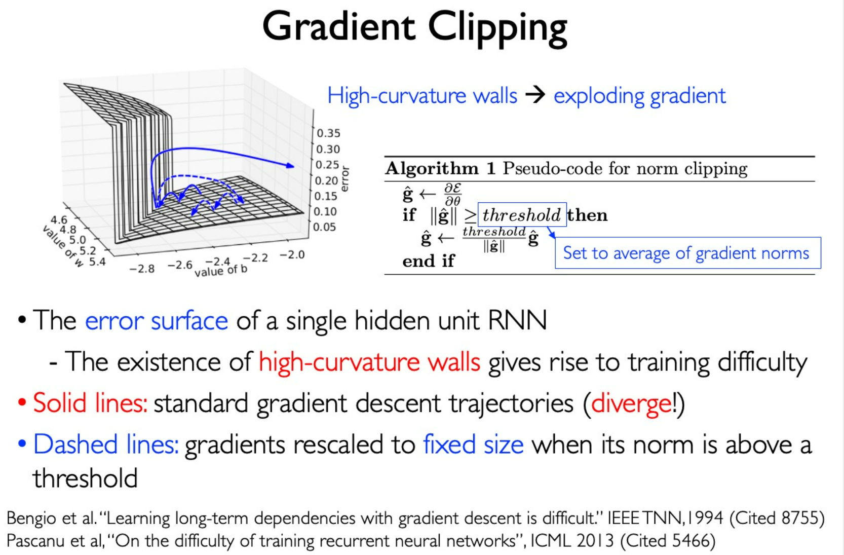
Problem: Gradient Explosion during continuously multiplication.
Solution: Gradient Clipping
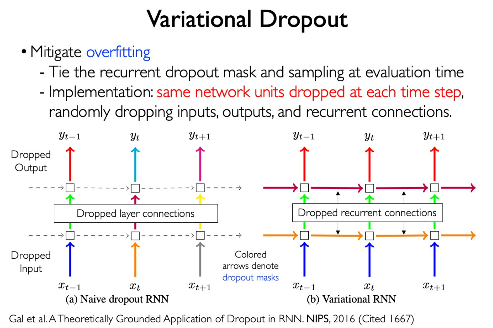
Variational Dropout
Layer Normalization
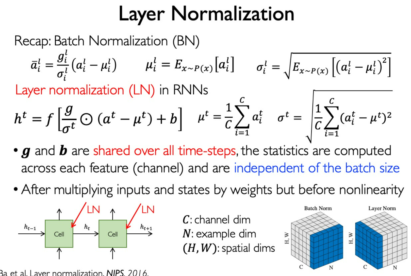
BN: Easy to compare between channels
LN: Easy to compare between samples
在图像任务上,我们一般认为 channel 之间的地位应该是相同的,因此常常采用 BN。
Transformer
use attention to replace state space.
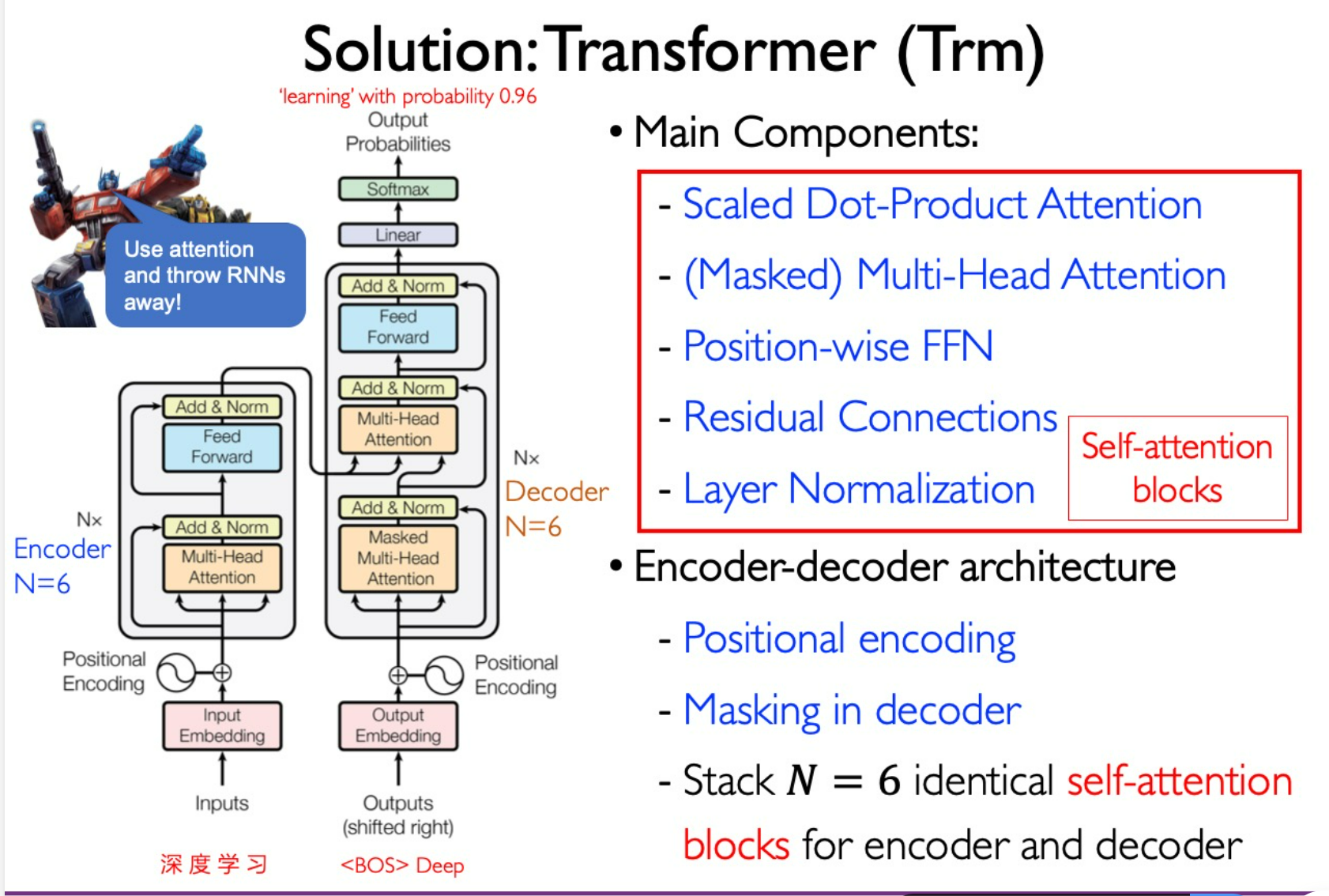
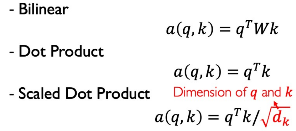
Attention
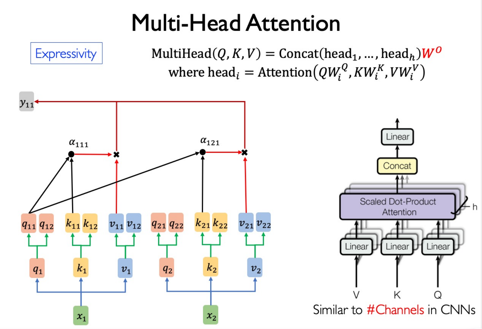
Multi-Head Attention
Sparse?
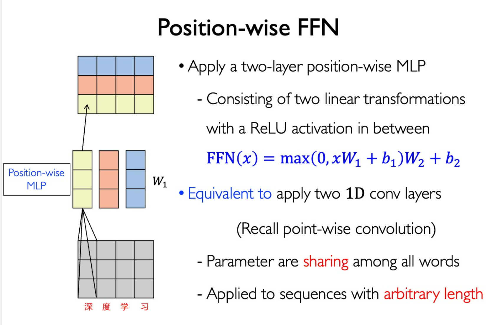
$W^o$ to maintain shape and jointly attend to information from different representation subspaces.FFN
Position-wise FFN (Similar to multi convolution kernels in CNN, shared parameters in every word.)
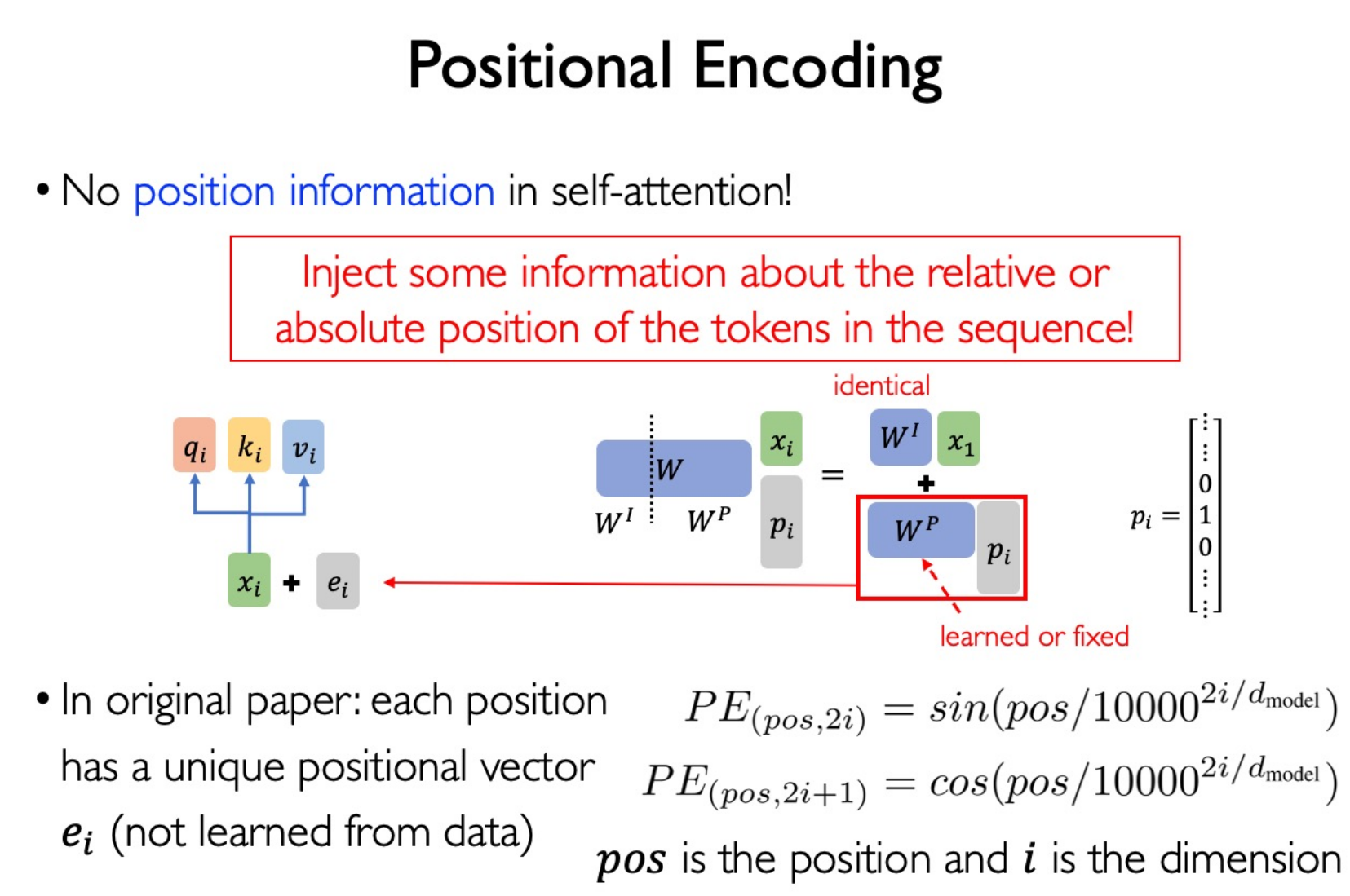
Positional Encoding
Reasoning
Reasoning (Probabilistic) = Modeling + Inference
Modeling:
- Bayesian Networks
- Markov random fields
Inference:
- Elimination methods (变量消除法)
- Latent variable models (因变量模型)
- Variational methods (变分方法)
- Sampling methods (采样方法) - 难学!
Bayesian Network
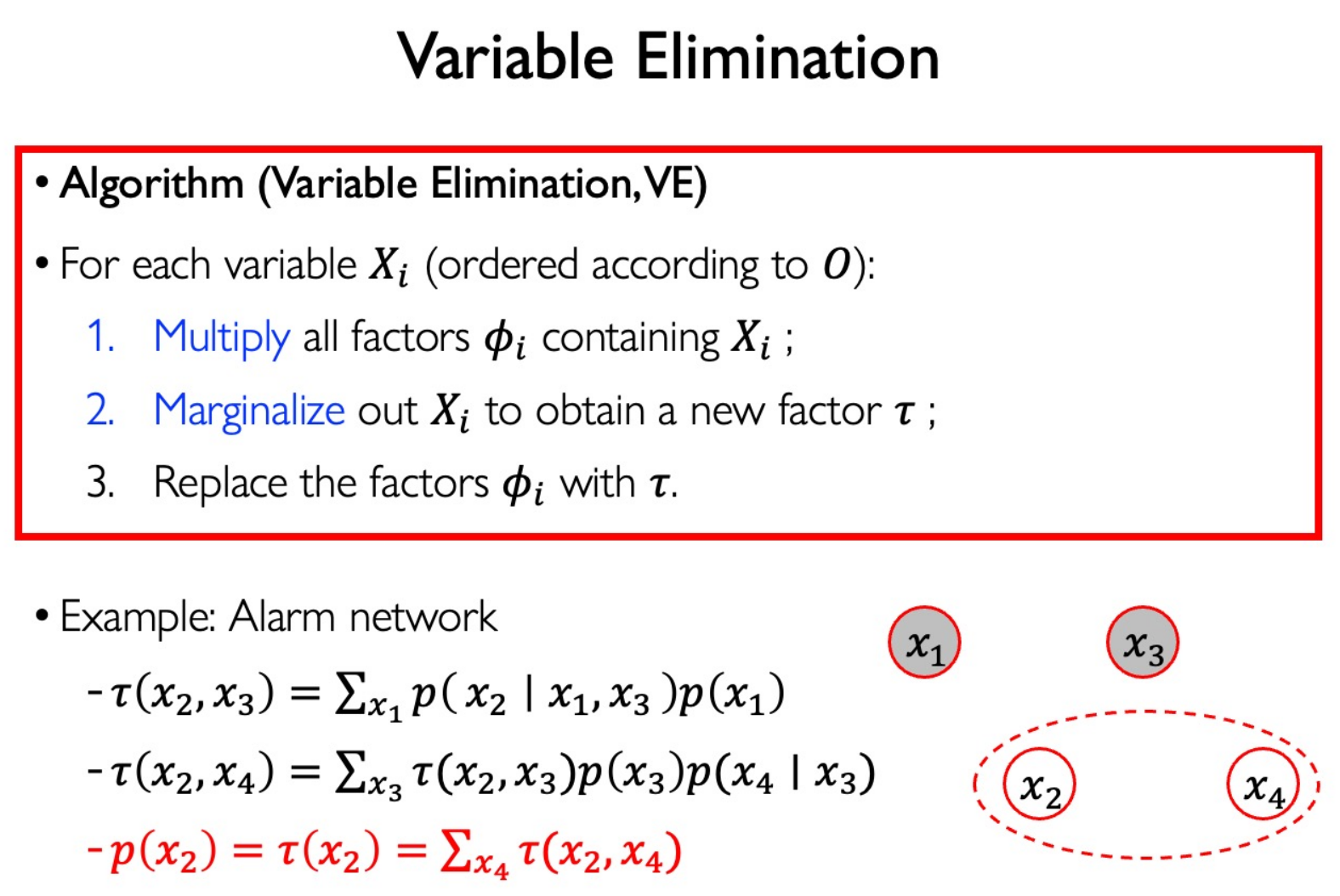
$$ p(x_1,...,x_K)=p(x_K|x_1,...,x_{K-1})\cdots p(x_2|x_1)p(x_1) $$Variable Elimination
用于计算概率的边缘分布
一般而言是 NP-hard 问题。
对于 Markov chain,复杂度为 $O(nk^2)$ ;对于一般的图, $O(k^{n-1})$ ;如果确定每个节点的父节点数不超过 m,则复杂度为 $O(nk^{m-1})$
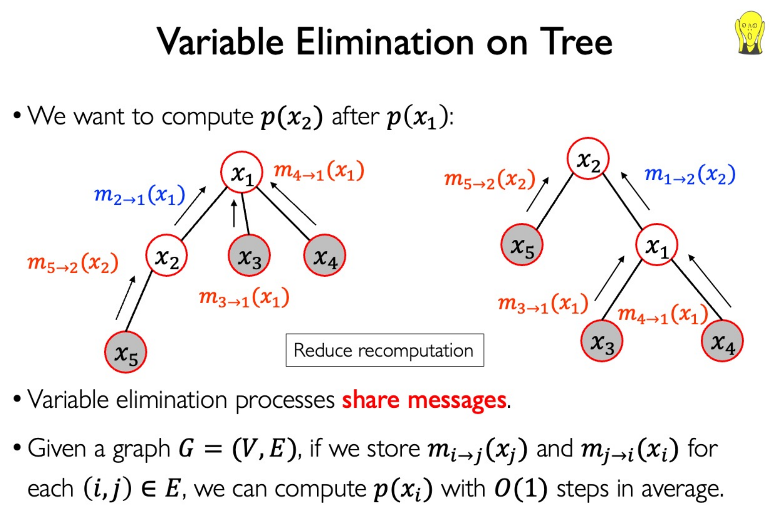
Message Passing
Reuse the computation from $P(Y|E=e)$ when calcuating another probability $P(Y_1|E_1=e_1)$
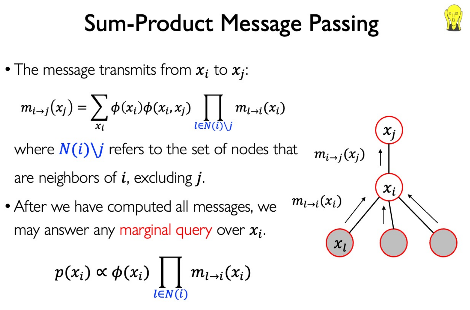
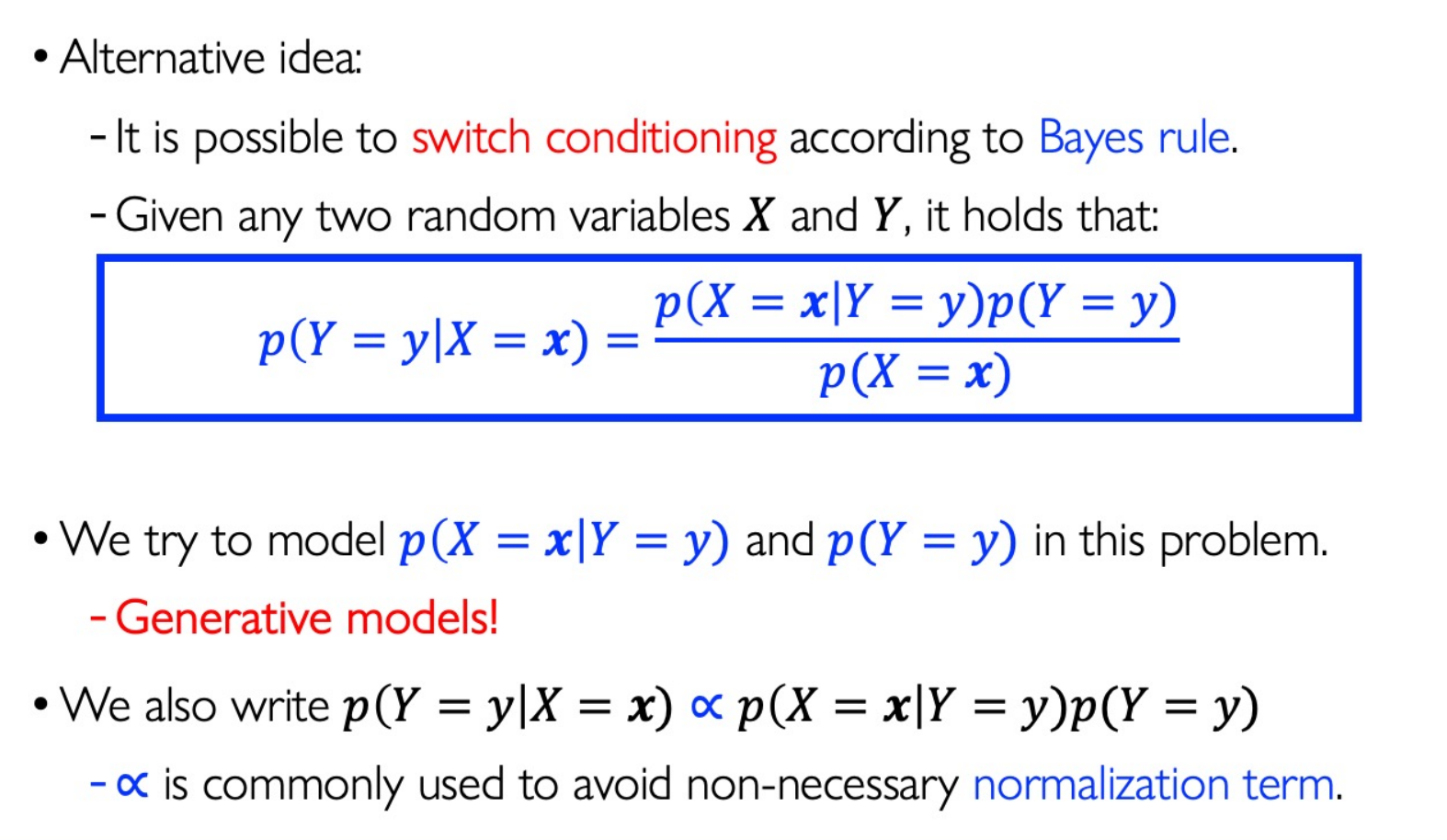
“ $\propto$ ” 意味着只需要知道概率的相对值就够了,因为可以通过归一化算出最终的概率值。
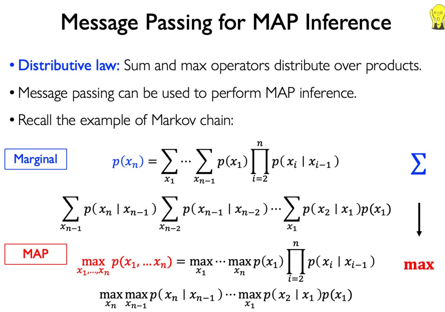
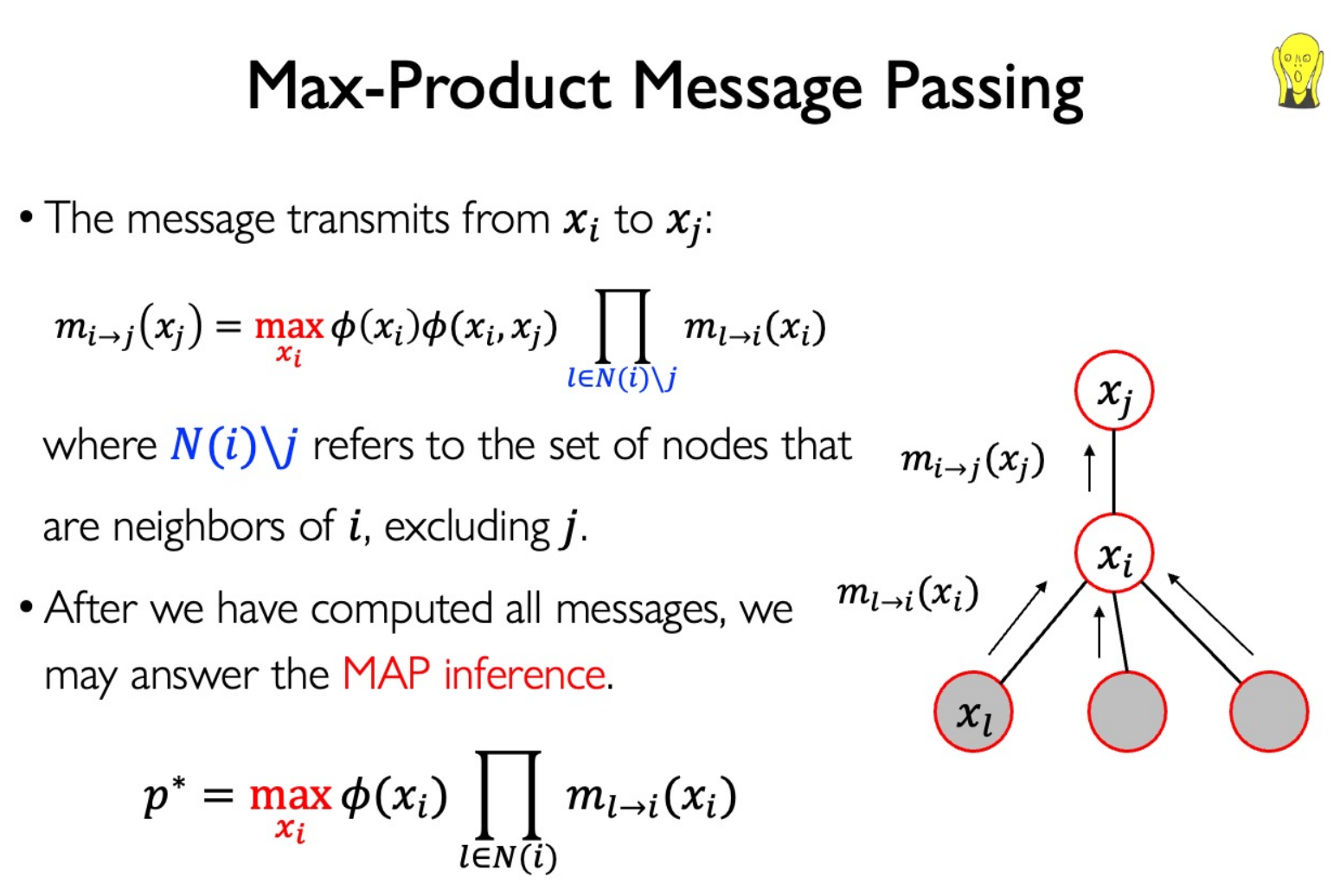
MAP 需要求概率分布的最大值。
sum 与 max 同为聚合操作,因此同样满足分配律,只需要对应替换就可以得到第二种 Message Passing:
Bayes Approach
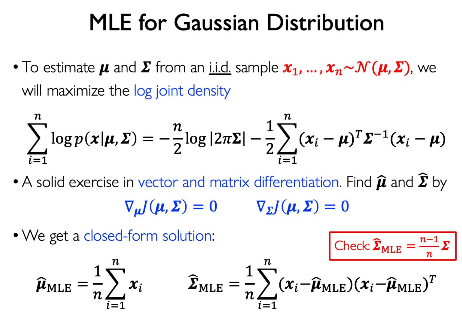
MLE method
如果概率模型的参数知道,称为概率;不知道,称为统计推断。
估计高斯分布的参数:
方差是有偏估计,所以一般× $1/(n-1)$ 。
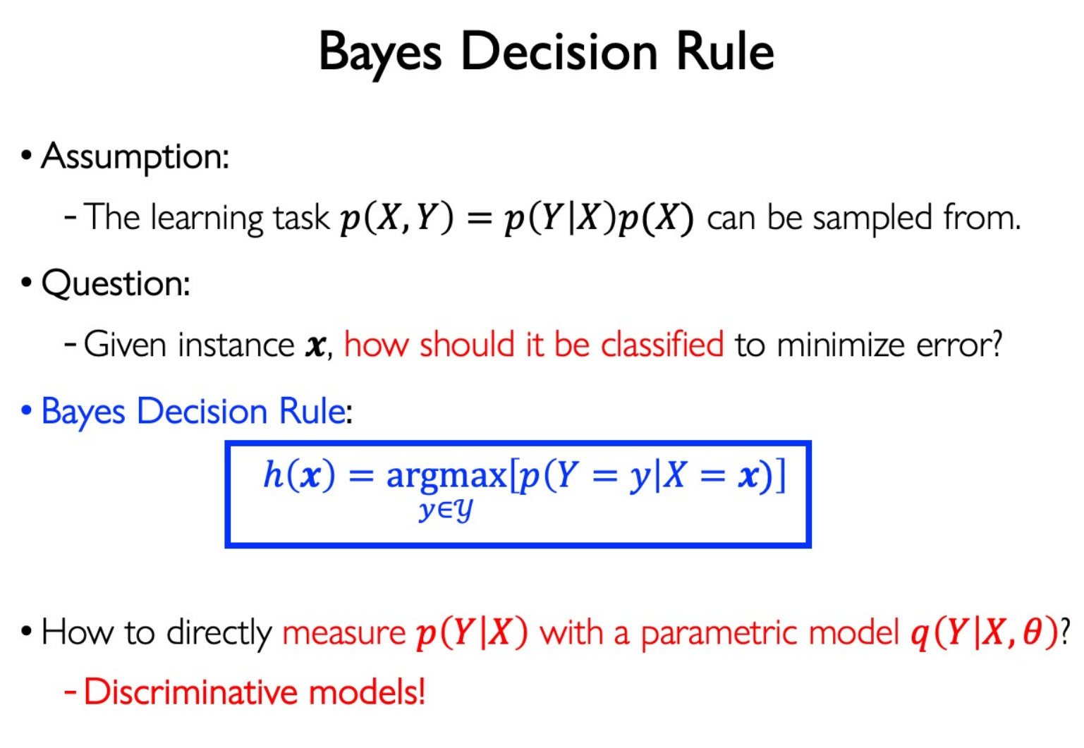
Bayes Decision Rule
对于回归问题,可以采用高斯噪声假设:
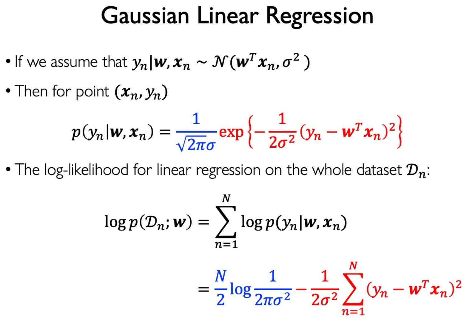
这样就得到了最小二乘估计。
MLE 是先验概率相等的 MAP。
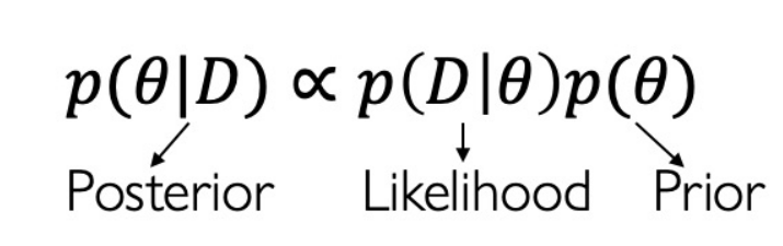
放在机器学习中,MAP 可以定义为:模型 = 数据 + 先验。
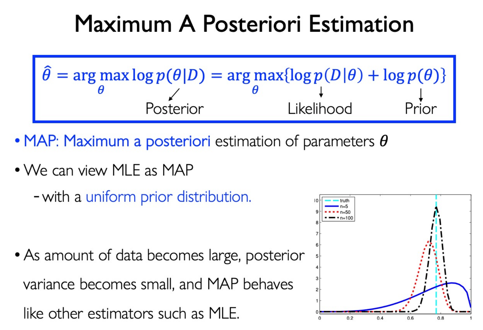
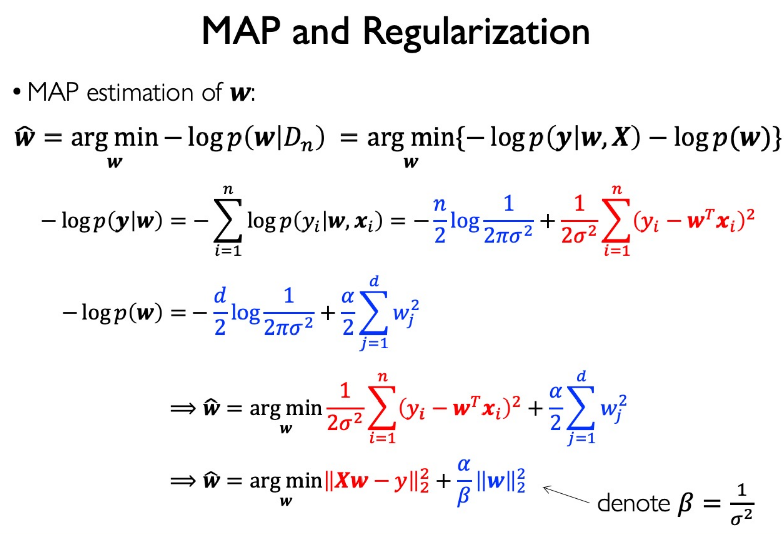
先验信息在机器学习中体现为正则化:
2 范数正则化就是在认为模型参数服从高斯分布的先验假设情况下,利用 MAP 准则来估计参数。
这也就是为什么正则化倾向于避免过拟合:高斯分布先验希望模型参数足够简单。
Bayesian Model Averaging
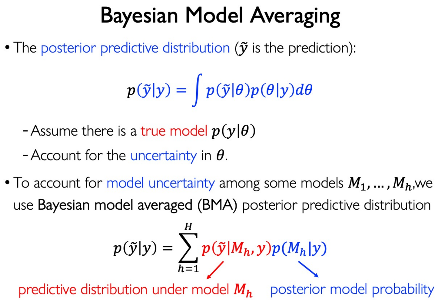
意义:模型集成。
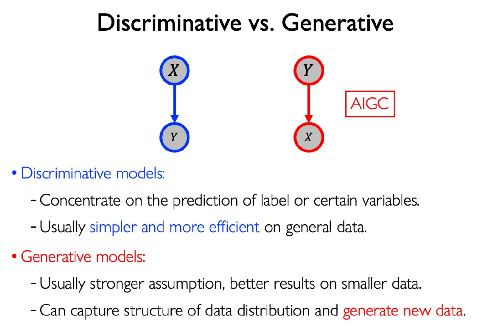
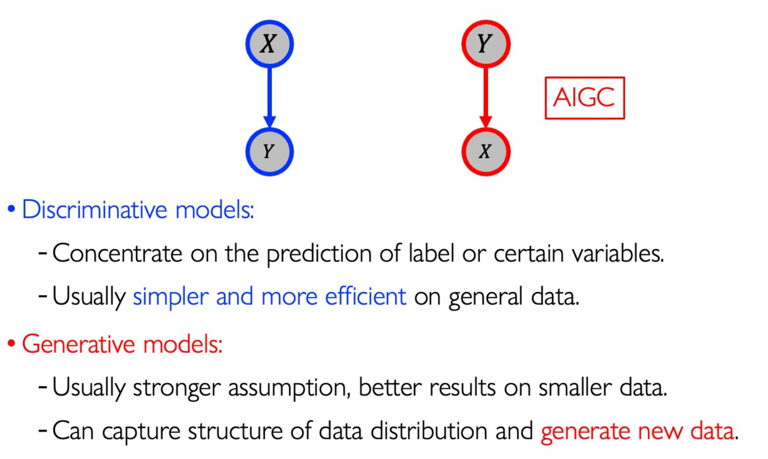
Discriminative Models
上面的理论足够解释判别式模型的原理了。
Generative Models
Naive Bayes Classifier
model $Y$ as a bernoulli distribution with parameters $p(y=1)$ and $p(y=-1)$
conditional independence: each dimension is independent given label y
$$ p(X=x|Y=y)=\prod_{j=1}^dp(x_{\cdot j}|y) $$Laplacian smoothing for 0 samples:
$$ p(x_{\cdot j}=r_j|Y=+1)=\frac{\sum_{i=1}^n1\{x_{\cdot j}=r_j\wedge y_i=+1\}+1}{\sum_{i=1}^n1\{y_i=+1\}+k_j} $$For dataset with all continuous features: descretize it, or use another model based on a different assumption.
Guassian Discriminant Analysis
是一个生成模型!虽然它被用来分类,但是它的建模设计上采用的是生成式。
For dataset with all continuous features:
Using parametrice distribution to represent $P(X=x|Y=y)$
A common assumption in classification:
- We always assume that data points in a class is a cluster.
Still model $p(Y=y)$ as Bernoulli distribution.
$$ \text{So we can model }p(X=x|Y=y)\text{ by Gaussian distribution:}\\p(X=x|Y=+1)\propto\exp\left(-\frac{1}{2}(x-\mu_{+})^{T}\Sigma^{-1}(x-\mu_{+})\right)\\p(X=x|Y=-1)\propto\exp\left(-\frac{1}{2}(x-\mu_{-})^{T}\Sigma^{-1}(x-\mu_{-})\right) $$Note the shared parameters $\Sigma$ for positive and nagative classes.
Use MLE to find the best solution:
$$ \ell(\phi,\mu_+,\mu_-,\Sigma)=\log\prod_{i=1}^np(x_i,y_i;\phi,\mu_+,\mu_-,\Sigma)\\=\log\prod_{i=1}^np(x_i|y_i;\mu_+,\mu_-,\Sigma)+\boxed{\log\prod_{i=1}^np(y_i|\phi)} $$Then:
$$ \phi=\frac{\sum_{i=1}^{n}1\{y_{i}=+1\}}{n},\mu_{+}=\frac{\sum_{i=1}^{n}1\{y_{i}=+1\}x_{i}}{\sum_{i=1}^{n}1\{y_{i}=+1\}},\mu_{-}=\frac{\sum_{i=1}^{n}1\{y_{i}=-1\}x_{i}}{\sum_{i=1}^{n}1\{y_{i}=-1\}}\\\boldsymbol{\Sigma}=\frac{1}{n}\boldsymbol{\Sigma}_{i=1}^{n}(\boldsymbol{x}_{i}-\boldsymbol{\mu}_{\boldsymbol{y}_{i}})(\boldsymbol{x}_{i}-\boldsymbol{\mu}_{\boldsymbol{y}_{i}})^{T} $$Discriminative vs. Generative
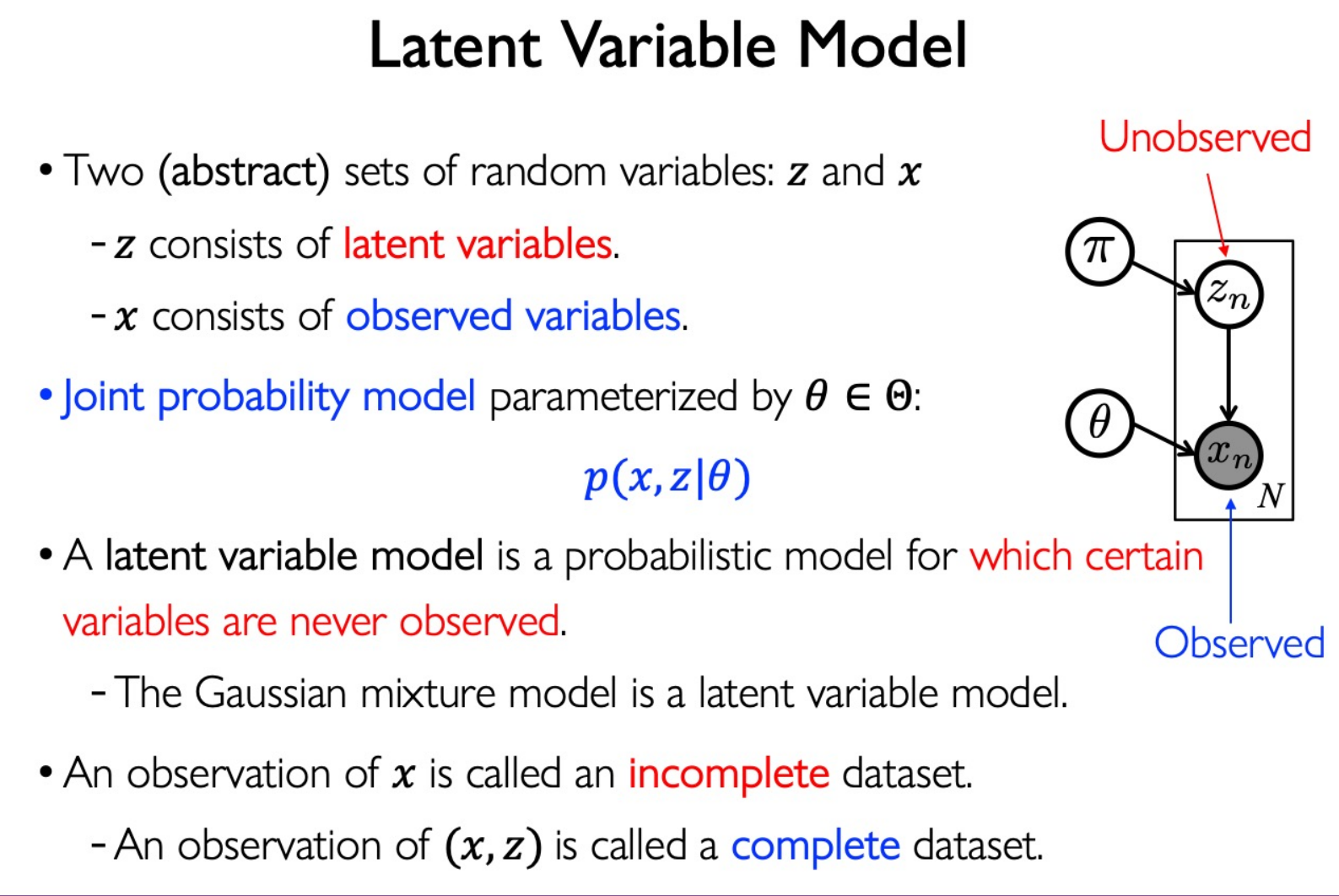
Mixture Models and EM
Gaussian Mixture Model
A Generative model. More assumption than Logistic Regression.
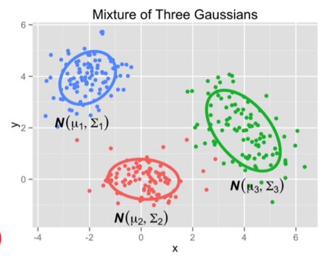
Sample dataset from GMM:
$$ p(x)=\sum_{z=1}^k\pi_z\mathcal{N}(x|\mu_z,\Sigma_z) $$Compute log-likelihood:
$$ \ell(\boldsymbol{\pi},\boldsymbol{\mu},\boldsymbol{\Sigma})=\log\prod_{i=1}^n\sum_{z=1}^k\pi_z\mathcal{N}(\boldsymbol{x}_i|\boldsymbol{\mu}_z,\boldsymbol{\Sigma}_z)=\sum_{i=1}^n\log\left[\sum_{z=1}^k\pi_z\mathcal{N}(\boldsymbol{x}_i|\boldsymbol{\mu}_z,\boldsymbol{\Sigma}_z)\right] $$ $$ \ell(\pi,\mu,\Sigma)=\sum_{i=1}^n\log\left[\sum_{z=1}^k\frac{\pi_z}{\sqrt{|2\pi\Sigma_z|}}\exp(-\frac12(x_i-\mu_z)^T\Sigma^{-1}(x_i-\mu_z))\right] $$Intracable! Use EM method to estimate parameters.
$z$ is latent variable.Expectation Maximization
Learing Problem:
find MLE
$$ \widehat{\theta}=\underset{\theta}{\operatorname*{argmax\ }}p(\mathcal{D}|\theta) $$Inference Promblem:
Given $x$ , find conditional variable of $z$ :
$$ p(z|x,\theta) $$EM method is for both problems!
it is hard to maximize the marginal likelihood directly:
$$ \max_\theta\log p(x|\theta) $$but the complete data log-likelihood is easy typically:
$$ \max_\theta\log p(x, z|\theta) $$if we had a distribution $q(z)$ for z:
$$ \max_\theta\sum_zq(z)\log p(x,z|\theta) $$We have Evidence Lower Bound (ELBO):
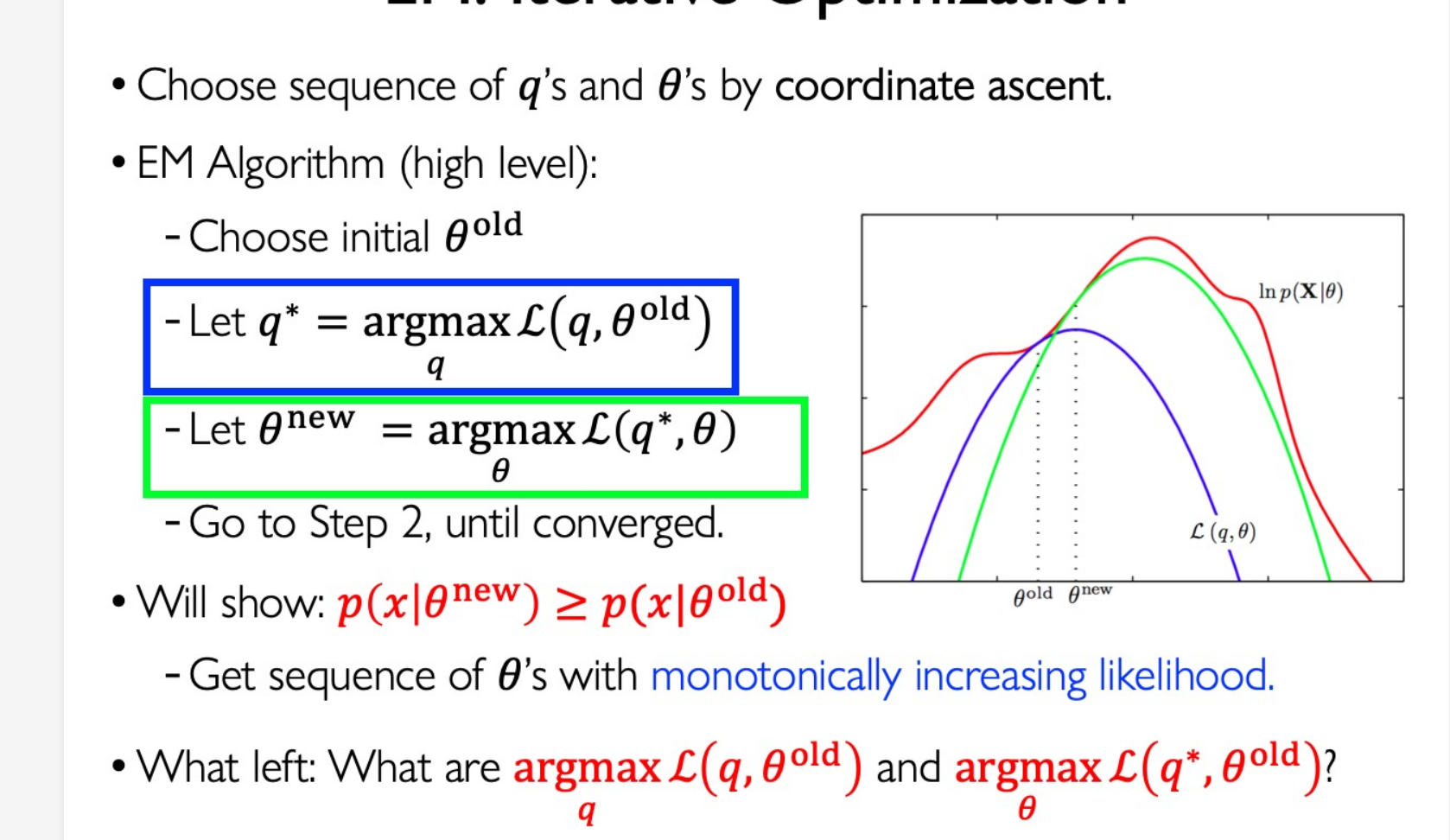
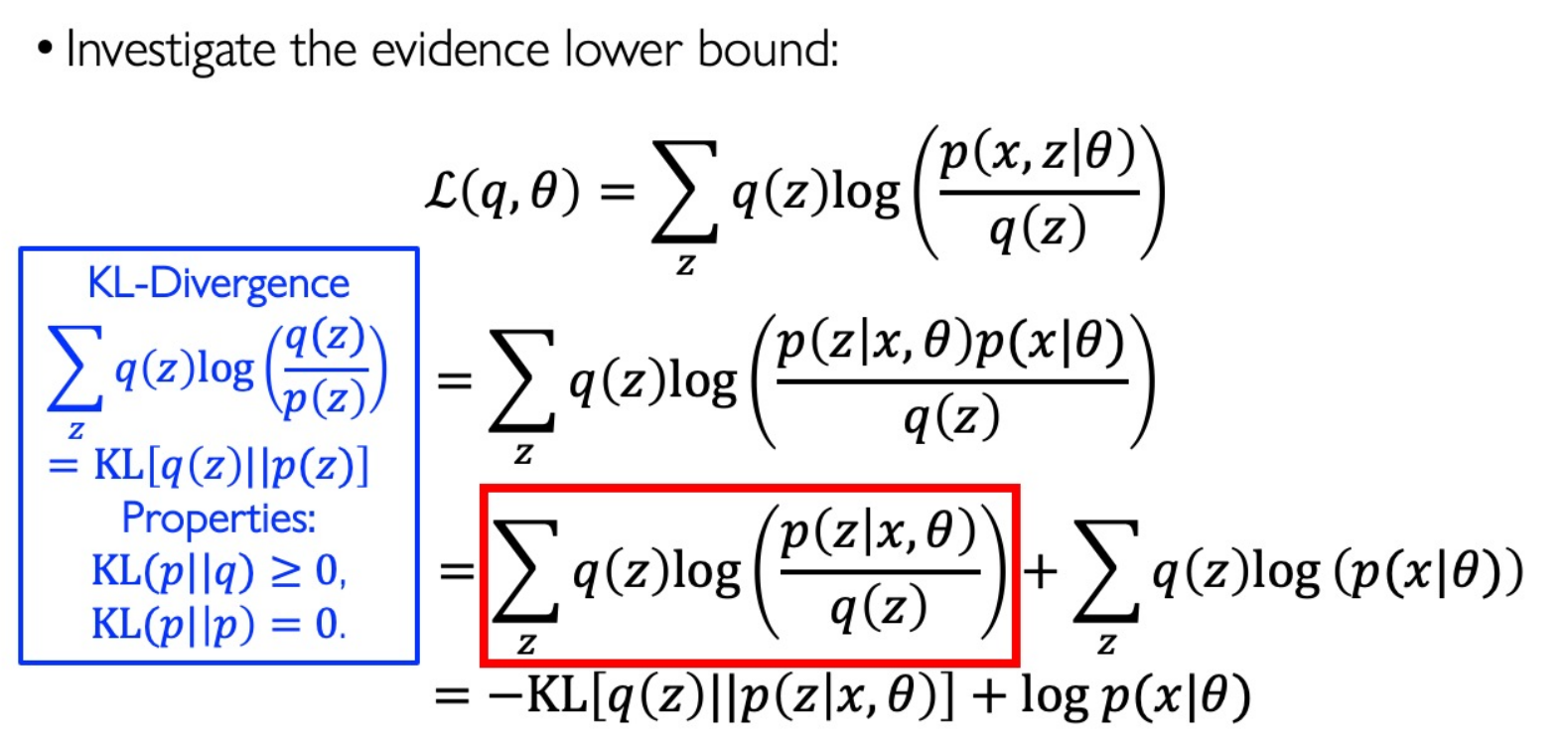
$$ \log p(x|\theta)=\log\left[\sum_zp(x,z|\theta)\right] \ge \underbrace{\sum_zq(z)\log(\frac{p(x,z|\theta)}{q(z)})}_{\mathcal{L}(q,\theta)} $$Now we optimize the ELBO iteratively:
The math background for ELBO:
We get back an equality for the marginal likelihood:
$$ \log p(x|\theta)=\mathcal{L}(q,\theta)+\mathrm{KL}[q(z)||p(z|x,\theta)] $$Evidence = ELBO + KL-Divergence
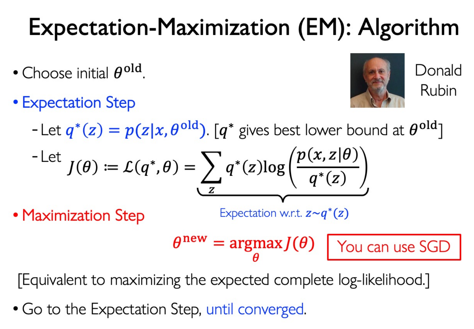
In E-step, if we want to maximize the ELBO without changing $\theta$ , we have to let KL be zero. Thus $q^*(z)=p(z|x,\theta)$
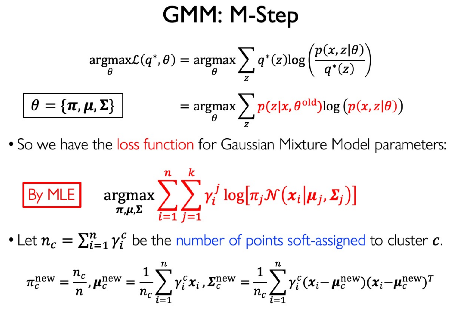
For M-step, we find the $\theta$ to maximize the ELBO.
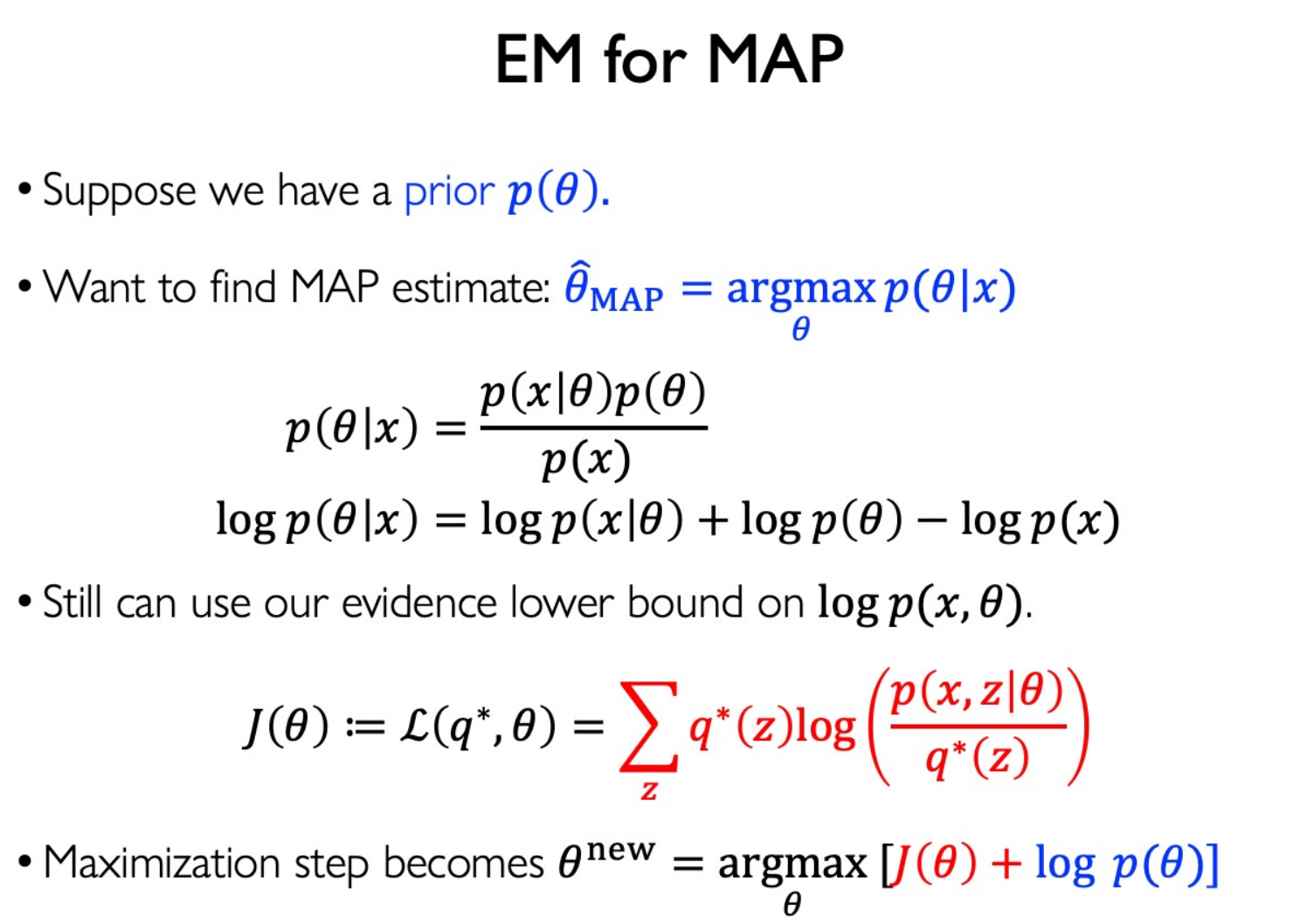
In MAP case:
For GMM, E-step:
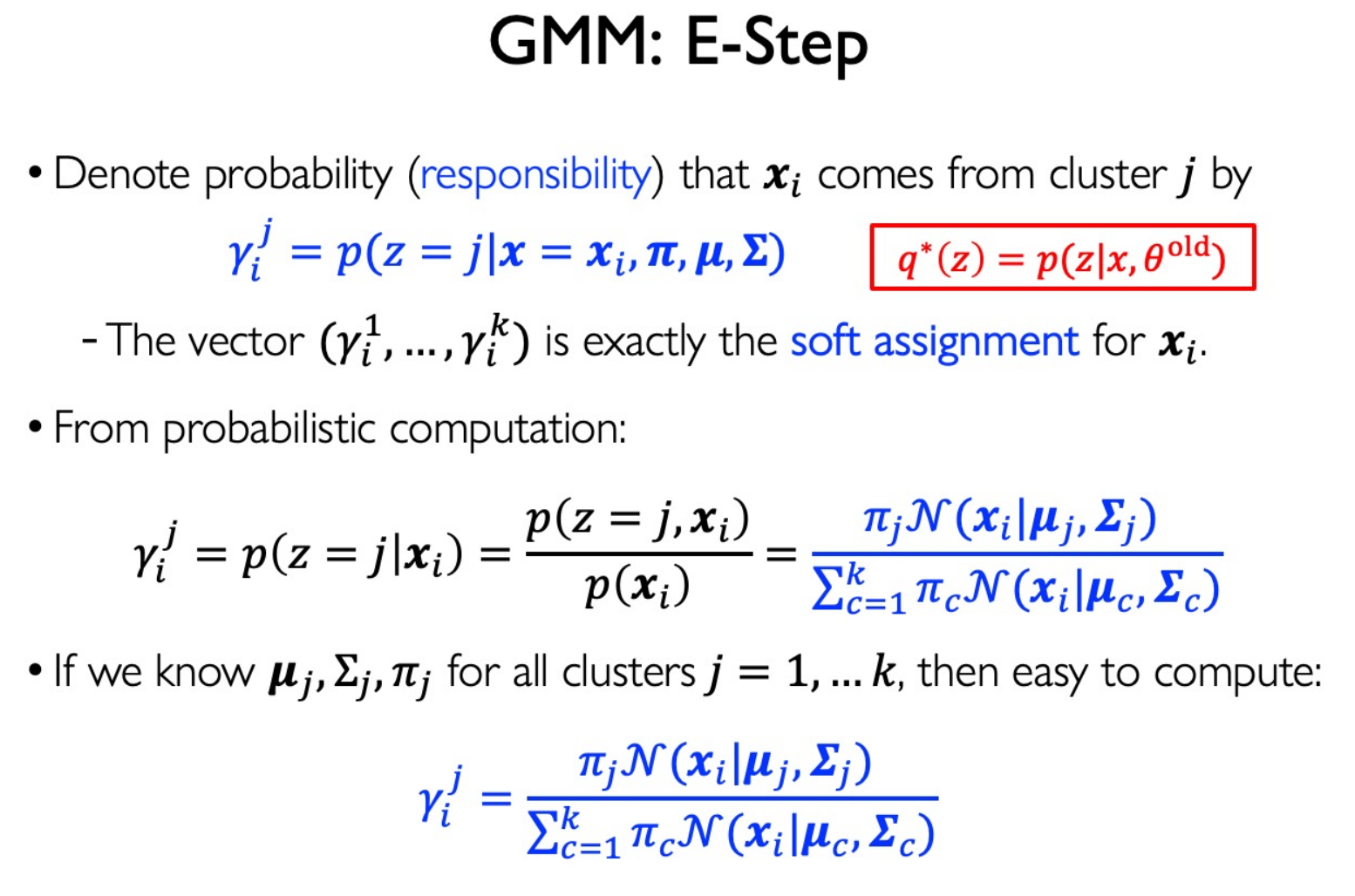
M-step:
Recommended Initialize:
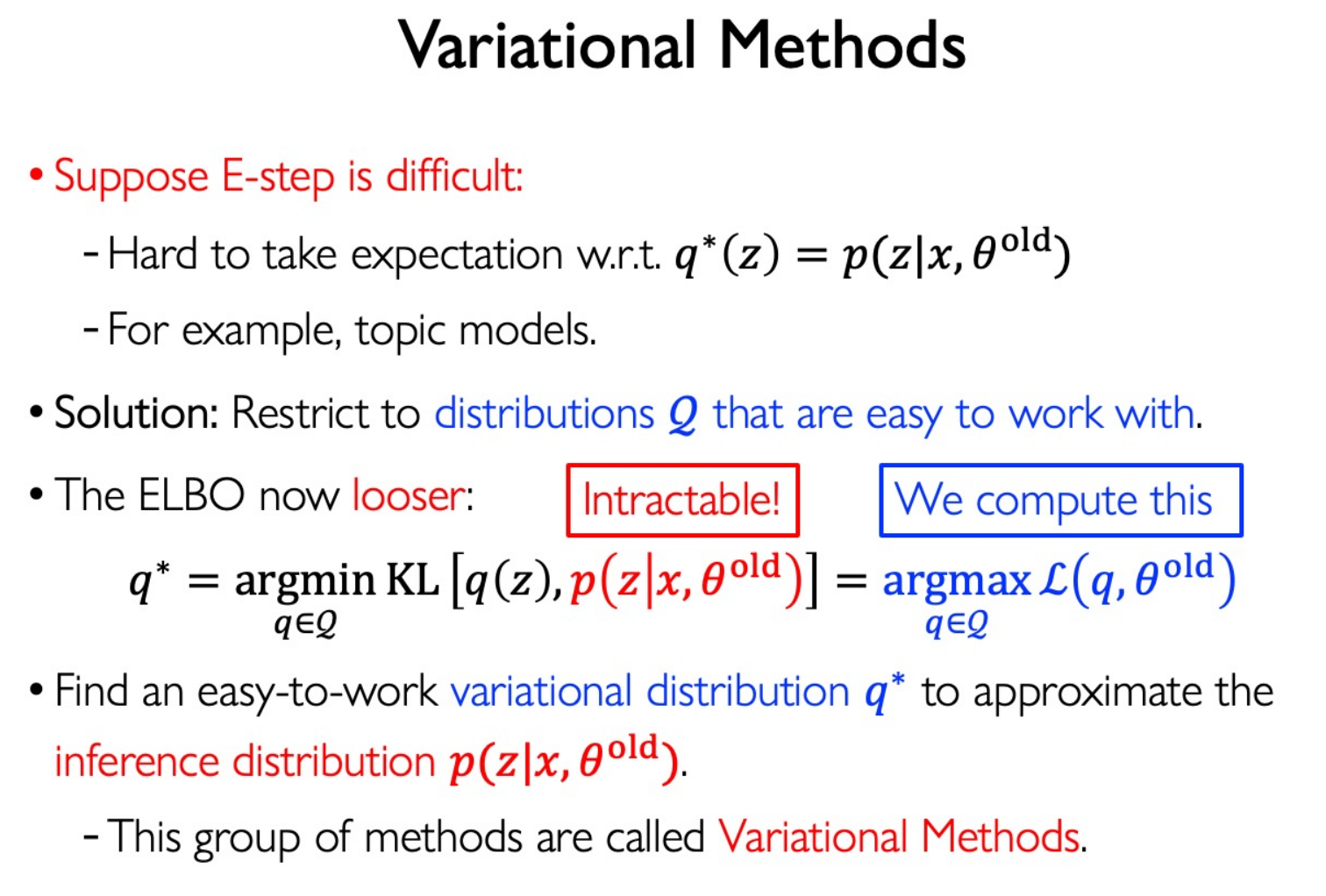
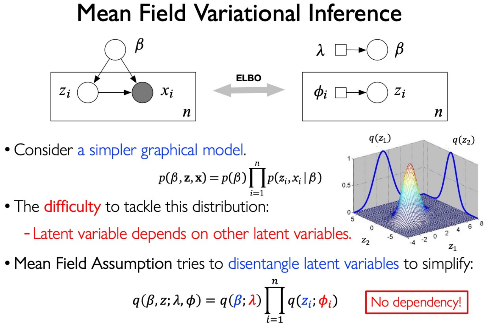
$$ \pi = 1/k\\ \mu = 0\\ \Sigma = \sigma^2 I $$Variational Methods:
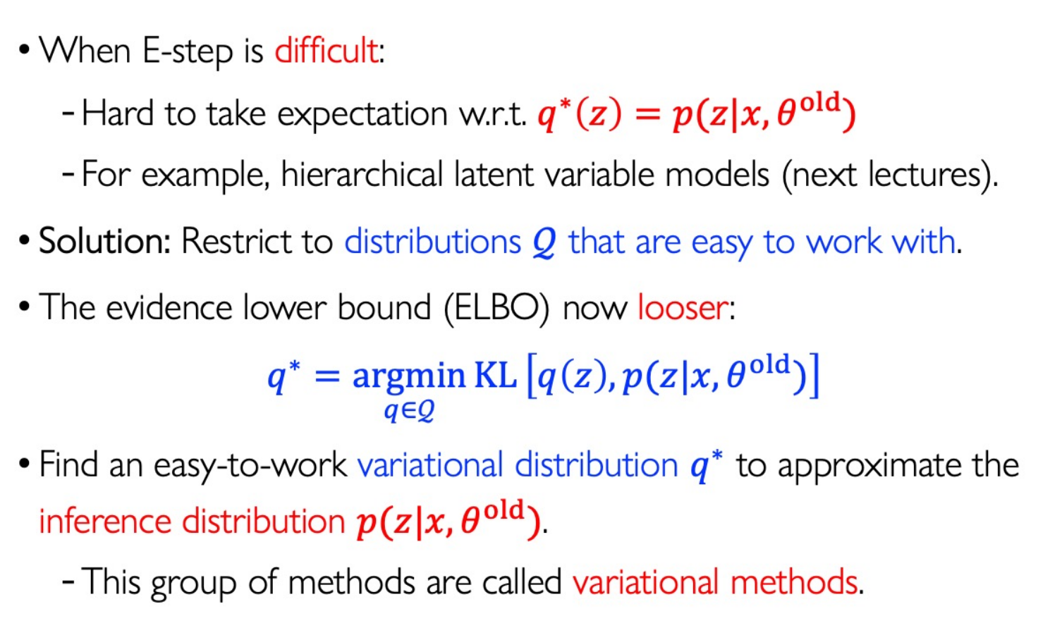
注意:E 步计算的是隐变量的后验(如果能计算出来),因为它是使得似然函数及ELBO最大的 $q(z)$ 。算不出来就用变分方法近似。
$q(z)$ 既不是先验分布,也不是后验分布,它只是我们对隐变量分布的一种估计。Probabilistic Topic Models
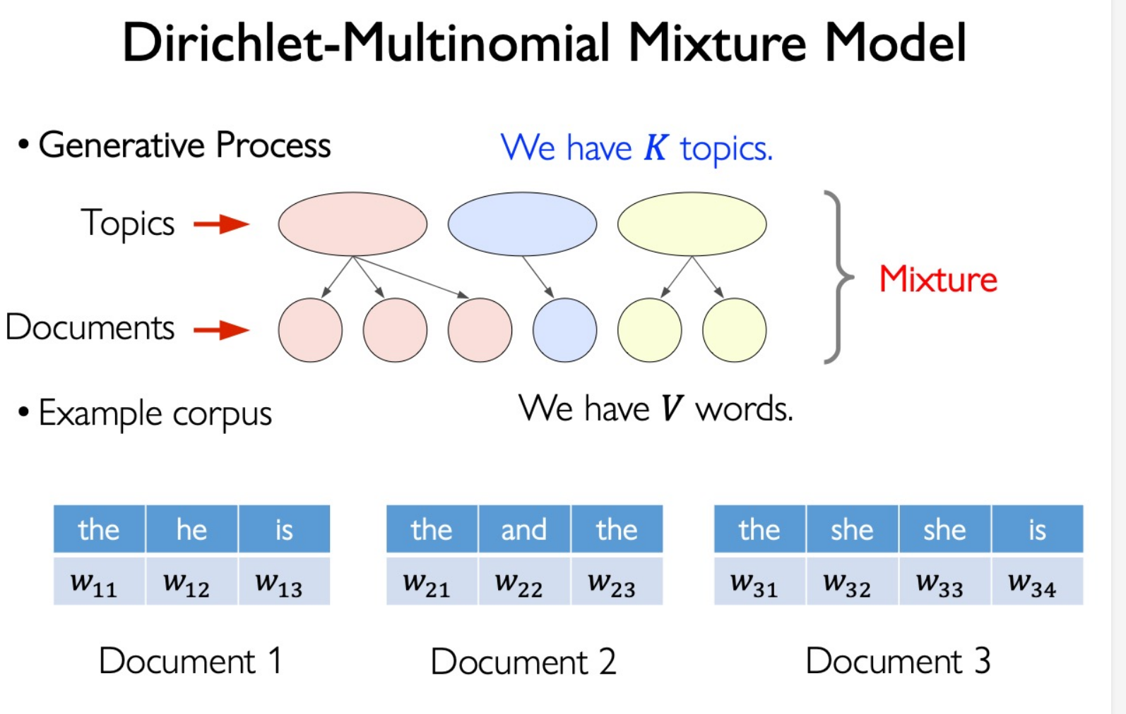
Dirichlet-Multinomial Model
Beta Distribution:
$$ f(\phi|\alpha,\beta)=\frac1{B(\alpha,\beta)}\phi^{\alpha-1}(1-\phi)^{\beta-1} $$Dirichlet Multinomial Model: Multi-dimensional version of Beta Distribution
$$ \boxed{p(\vec{\theta}|\boldsymbol{\alpha})}=\frac1{B(\boldsymbol{\alpha})}\prod_{k=1}^K\theta_k^{\alpha_k-1}\quad\text{Where }B(\alpha)=\frac{\Pi_{k=1}^K\Gamma(\alpha_k)}{\Gamma(\sum_{k=1}^K\alpha_k)} $$Conjugate prior:
$$ \sum_{i=1}^K\theta_i=1 $$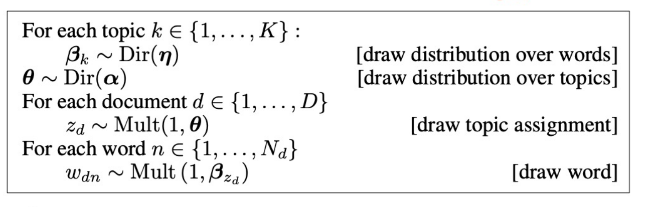
Admixture:
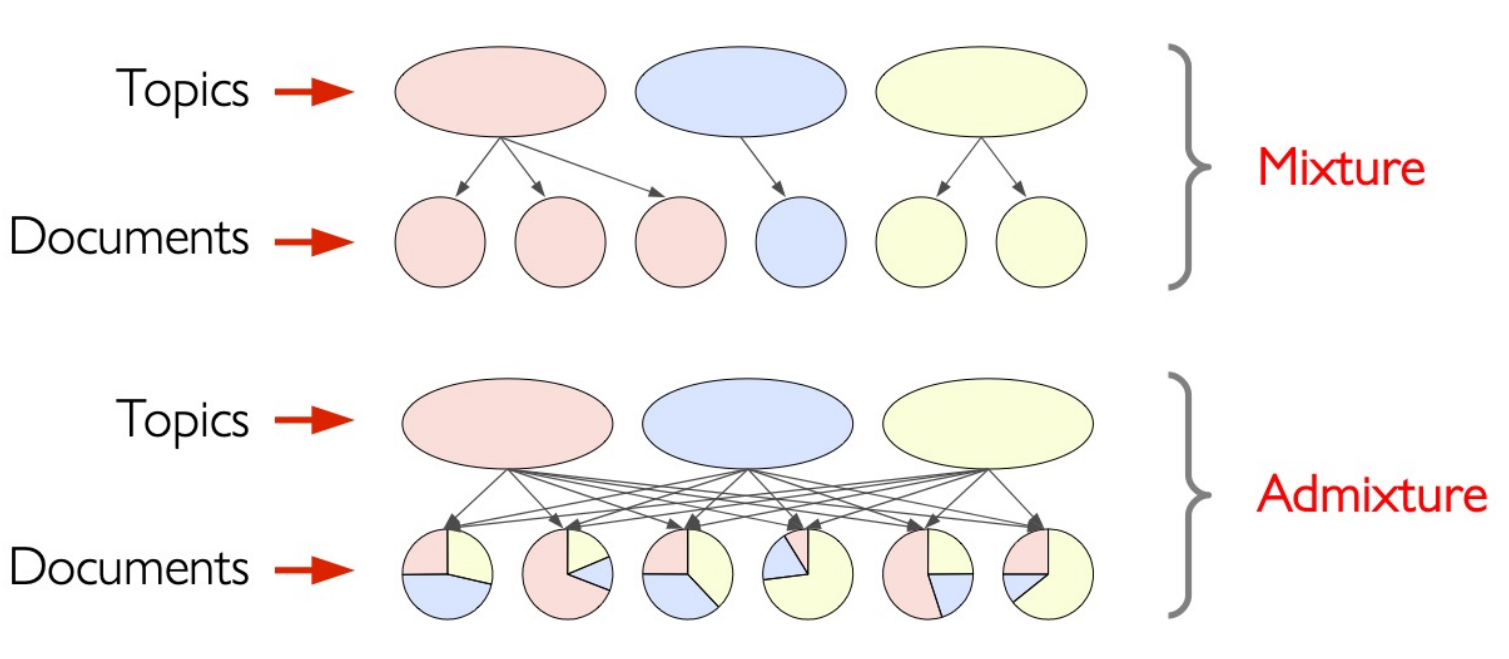
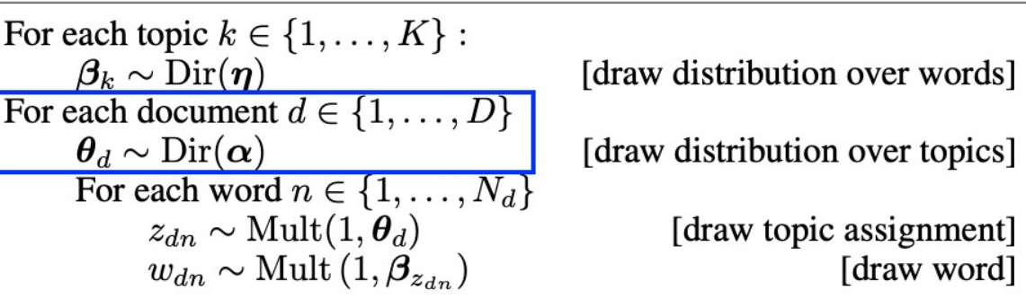
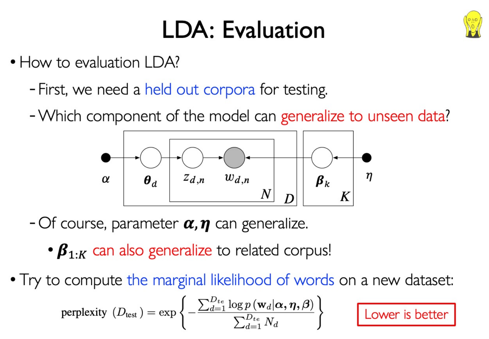
Latent Dirichlet Allocation (LDA):
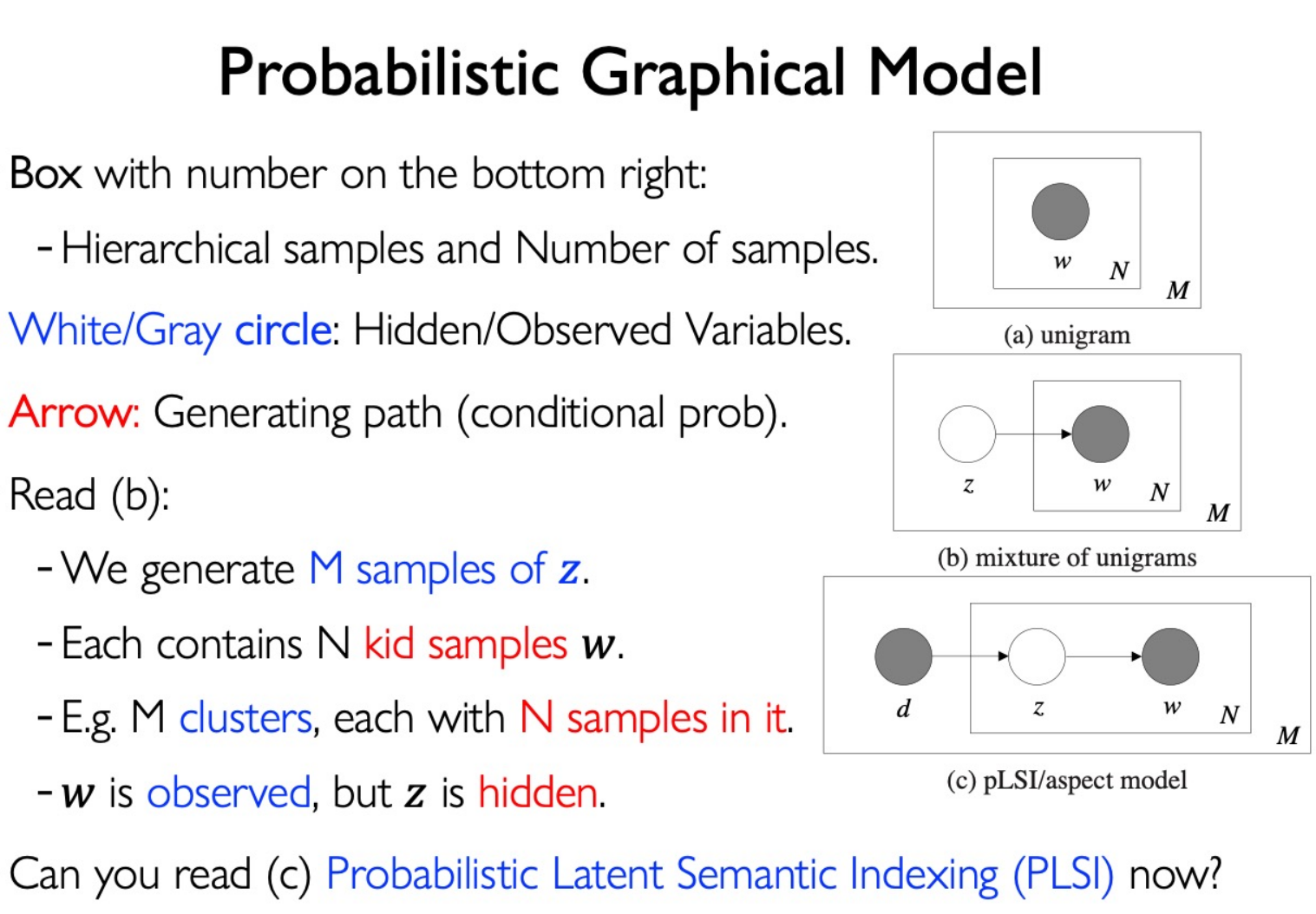
Probabilistic Graphical Models:
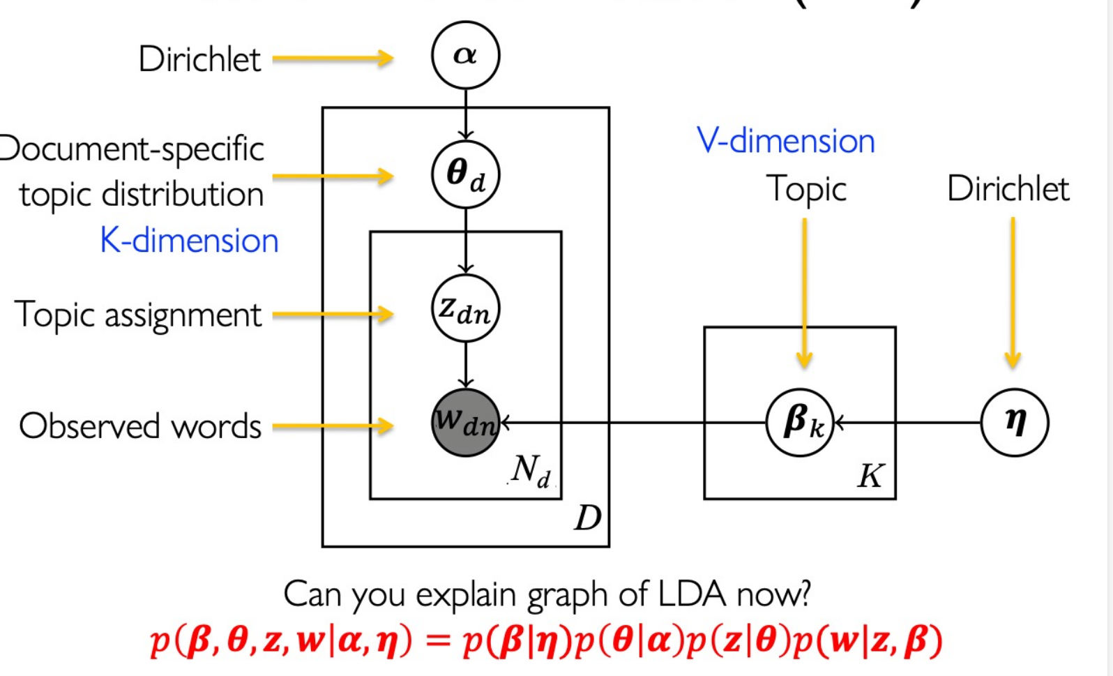
Maximum Likelihood Estimation
$$ \log p(\beta,\theta,z,w|\alpha,\eta)\\ =\sum_{k=1}^K\log p(\vec{\beta}_k|\eta)+\sum_{d=1}^D\log p(\vec{\theta}_d|\alpha)+\sum_{d=1}^D\sum_{n=1}^{N_d}\log p(z_{d,n}|\vec{\theta}_d)\\ +\sum_{d=1}^D\sum_{n=1}^{N_d}\log p(w_{d,n}|z_{d,n},\vec{\boldsymbol{\beta}}_{1:K})\\ \begin{aligned} &=\sum_{k=1}^{K}\left(\sum_{v=1}^{V}(\eta_{v}-1)\log\beta_{kv}-\log B(\eta)\right)+\sum_{d=1}^{D}\sum_{k=1}^{K}(\alpha_{k}-1)\log\theta_{dk}-\log B(\alpha) \\ &+\sum_{d=1}^D\sum_{n=1}^{N_d}\log\theta_{d,z_{d,n}}+\sum_{d=1}^D\sum_{n=1}^{N_d}\log\beta_{z_{d,n}w_{d,n}} \end{aligned} $$To learn the param $\alpha, \eta$ , use EM method:
In E-step, calculate
$$ q^*(z)=p(z|x,\theta^{\mathrm{old}}) $$ $$ p(\theta,z,\beta\mid w,\alpha,\eta)=\frac{p(\theta,z,\beta,w\mid\alpha,\eta)}{p(w\mid\alpha,\eta)} $$However, the denominator is intractable:
$$ p(\mathbf{w}|\alpha,\eta)=\int\int\sum_\mathbf{z}p(\boldsymbol{\theta},\mathbf{z},\boldsymbol{\beta},\mathbf{w}|\boldsymbol{\alpha},\boldsymbol{\eta})d\boldsymbol{\theta}d\boldsymbol{\beta} $$This problem is for general Bayesian models. We can use Variational Methods or Markov Chain Monte Carlo to solve it.
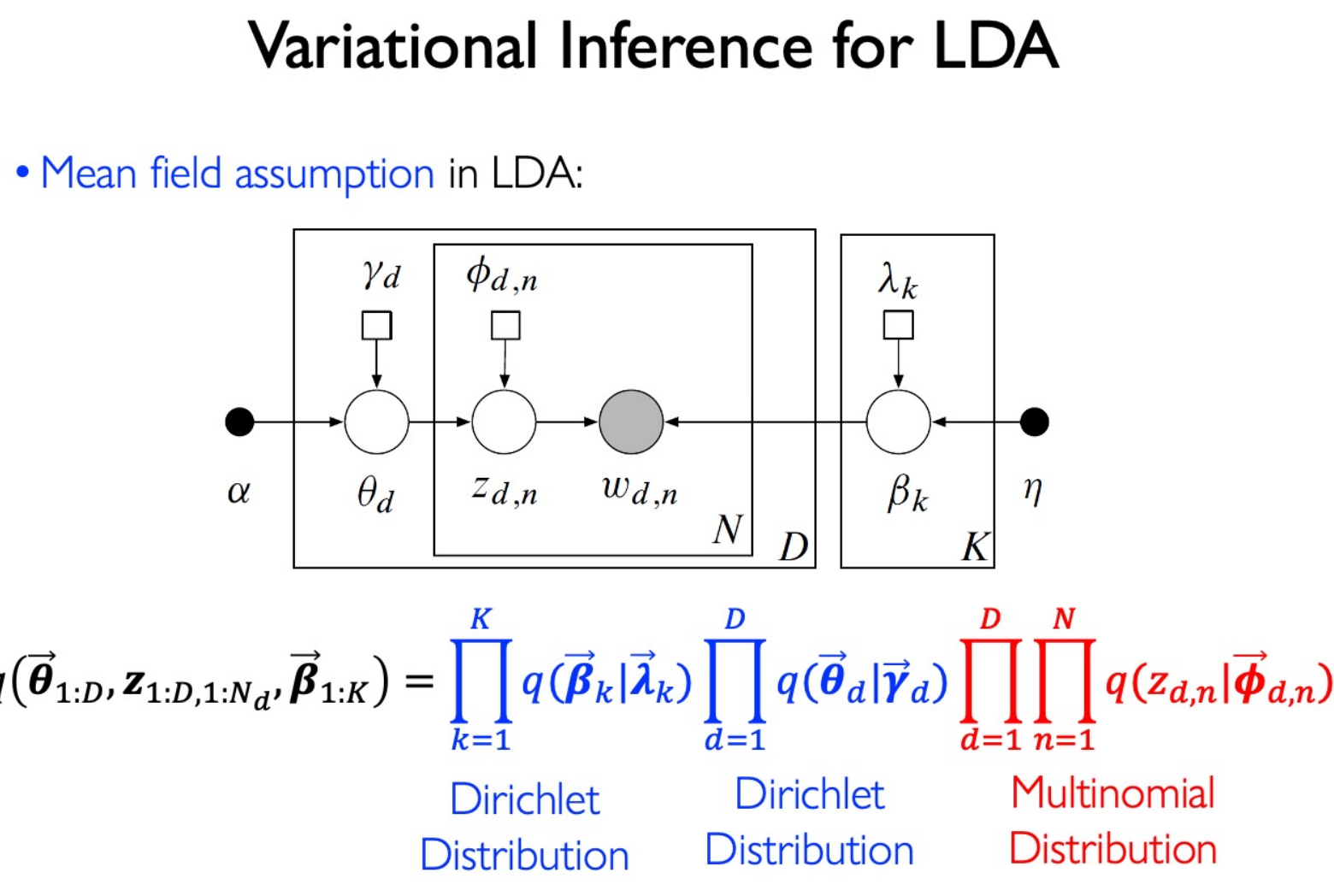
Variational Methods
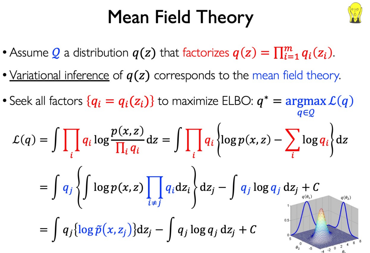
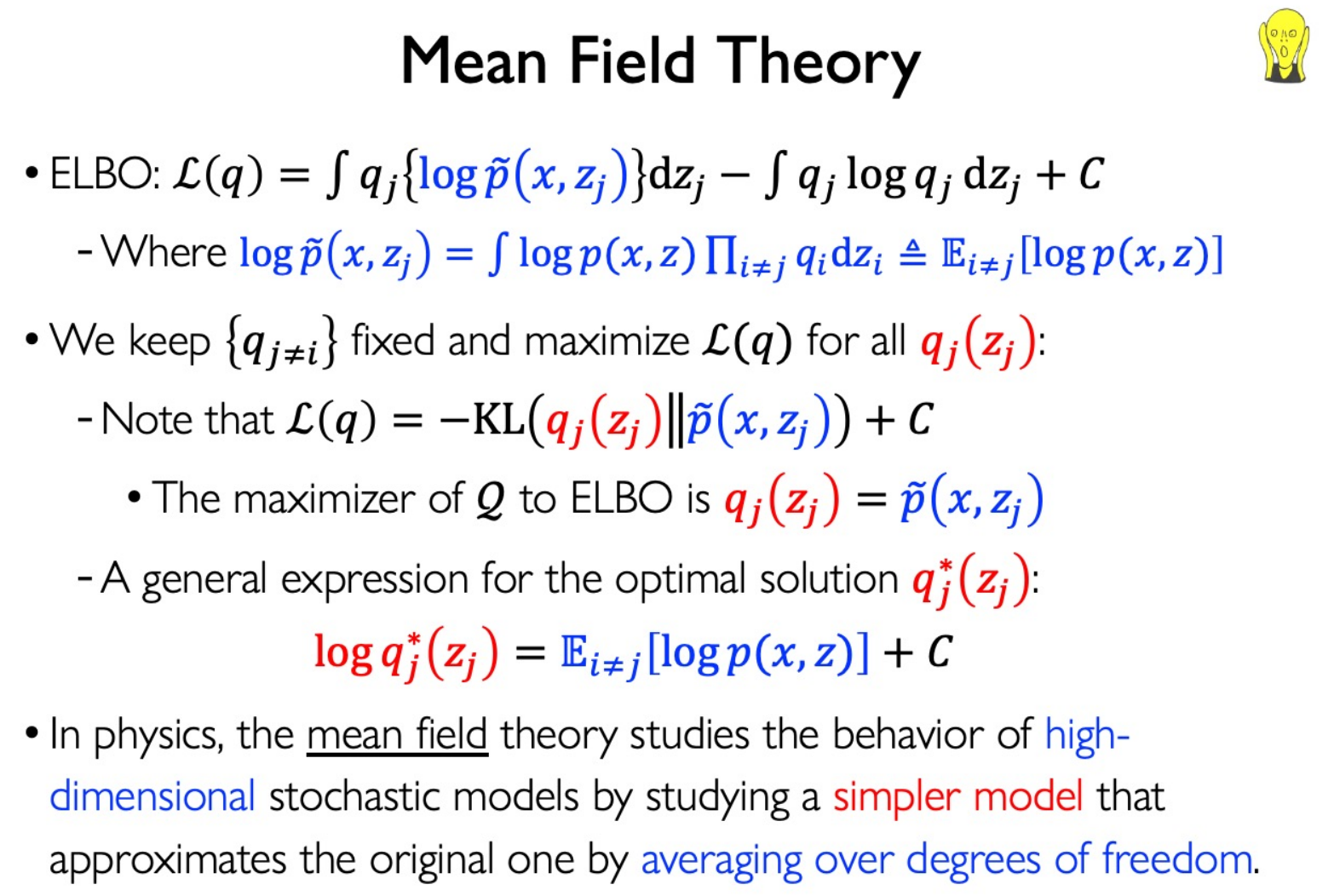
Use Mean field assumption in LDA:
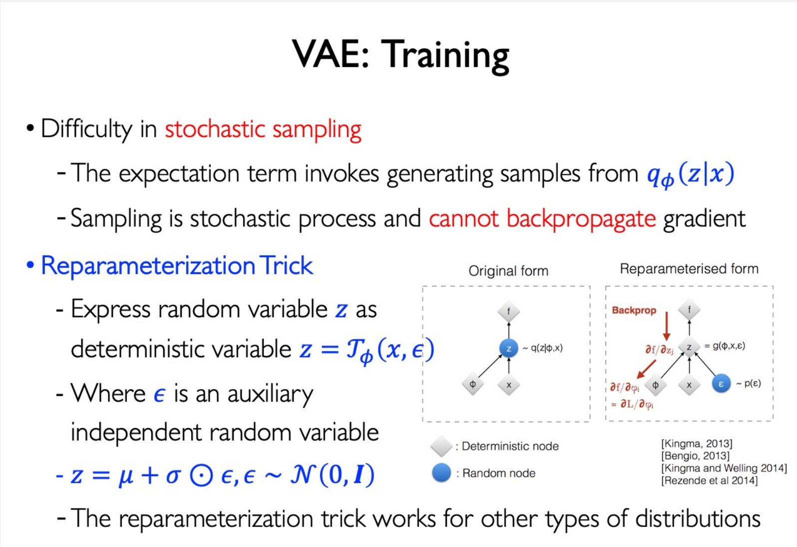
Variational Autoencoders (VAE)
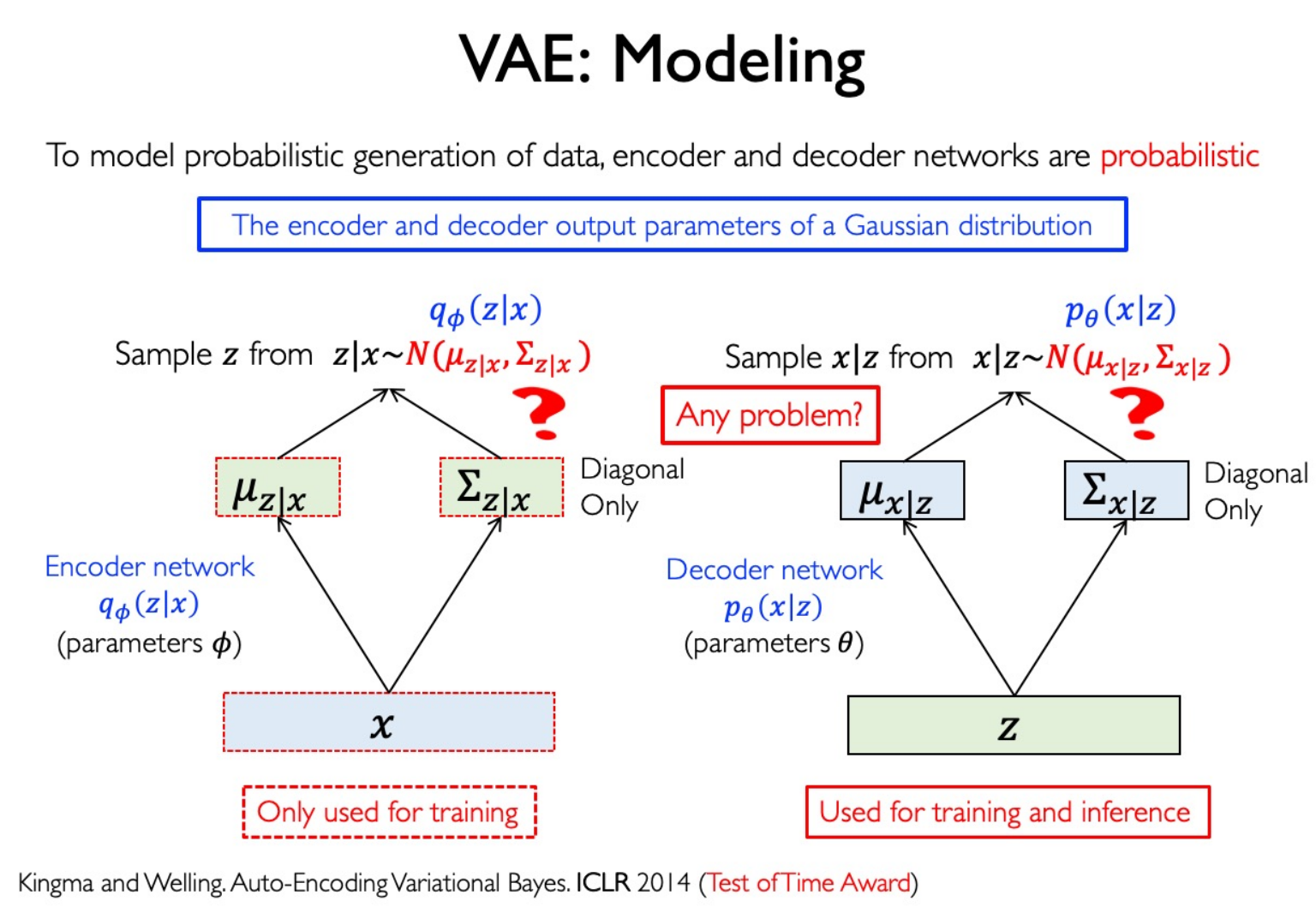
Reparameterization Trick: