Principle of Antenna

Introduction of Antenna

Definition of Antenna

• Transmitter and receiver of EM wave
• Signal from current to wave
• from lumped to distributed

Antenna classifications

• Resonant and non-resonant/leaky/travelling wave
• Antenna number: element, multiple antennas, array
• Shape: wire, loop, slot, patch/microstrip, cavity
• Materials: metallic, dielectric
• Property: wideband, narrow band
• Yagi-Uda, Vivaldi, Cassegrain
• Function: moblie/handset, base station, AiP

Maxwell equations

$$ \nabla \cdot \vec D = \rho \rightarrow \nabla \cdot \tilde{\vec D} = \rho \\ \nabla \cdot {\vec B} = 0 \rarr \nabla \cdot \tilde{\vec B} = 0\\ \nabla \times {\vec E} = -\frac{\partial \vec B}{\partial t} \rarr \nabla \times \tilde{\vec E} = -j\omega \tilde{\vec B}\\ \nabla \times {\vec H} = \vec J + \frac{\partial \vec D}{\partial t} \rarr \nabla \times \tilde{\vec H} = \vec J + j\omega \tilde{\vec D}\\ \vec D = \varepsilon \vec E\\ \vec B = \mu \vec H $$ $$ \nabla^2 \vec F = \nabla(\nabla \cdot \vec F) - \nabla \times (\nabla \times \vec F)\\ \nabla \times (\nabla f) = 0\\ \nabla \cdot (\nabla \times \vec F) = 0 $$

Auxiliary Potential Functions

Let

$$ \vec B = \nabla \times \vec A\\ \vec E + j\omega \vec A = -\nabla \phi $$ $$ \nabla \cdot \vec D = \varepsilon \nabla \cdot(-\nabla \phi - j\omega \vec A) = \rho\\ \Rightarrow \nabla^2\phi + \omega^2\mu\varepsilon\phi = - \frac{\rho}{\varepsilon} - j\omega(\nabla \cdot \vec A + j\omega \mu \varepsilon \phi) $$ $$ \nabla \times \vec H = \frac{1}{\mu}(\nabla(\nabla \cdot \vec A) - \nabla^2\vec A) = \vec J + j\omega \vec D = \vec J + j\omega\varepsilon(-\nabla\phi - j\omega \vec A)\\ \Rightarrow \nabla^2\vec A + \omega^2\mu\varepsilon\vec A = -\mu \vec J - \nabla(\nabla \cdot \vec A + j\omega\mu\varepsilon\phi) $$

Use Lorentz Gauge

$$ \nabla \cdot \vec A + j\omega\mu\varepsilon\phi = 0 $$

Then

$$ \nabla^2\vec A + \omega^2\mu\varepsilon\vec A = -\mu \vec J\\ \nabla^2\phi + \omega^2\mu\varepsilon\phi = - \frac{\rho}{\varepsilon} $$

Solve ODE:

$$ \begin{equation} \nabla^2\phi + k^2\phi = 0(r\ne 0) \end{equation}\\ \begin{equation} \nabla^2\phi + k^2\phi = -\frac{\rho}{\varepsilon}(r=0) \end{equation} $$

For (1)

$$ u(r) = \frac{\phi(r)}{r}\\ \frac{\rm{d}^2}{\rm{d}r^2}u + k^2u = 0\\ u = C_1e^{-jkr} + C_2e^{jkr}\\ \phi = C_1\frac{e^{-jkr}}{r} $$

For (2), in arbitrary volume

$$ \iiint_V(\nabla^2\phi + k^2\phi)\mathrm dv = \iiint_V(-\frac{\rho}{\varepsilon}\mathrm dv) = -\frac{q}{\varepsilon}\\ r \rightarrow 0\\ \iiint_V(k^2\phi)\mathrm dv = 0\\ \iiint_V\nabla^2\phi \mathrm dv = \oiint_S \nabla\phi \cdot \mathrm d\vec s = C_1 \oiint_S (\frac{-jkre^{-jkr} - e^{-jkr}}{r^2})\mathrm d\vec s = C_1 (\frac{-jkre^{-jkr} - e^{-jkr}}{r^2})4\pi r^2 = -C_1 4\pi $$

Finally,

$$ \phi(r) = \frac{q}{4\pi\varepsilon}\frac{e^{-jkr}}{r} $$

Radiation Parameters

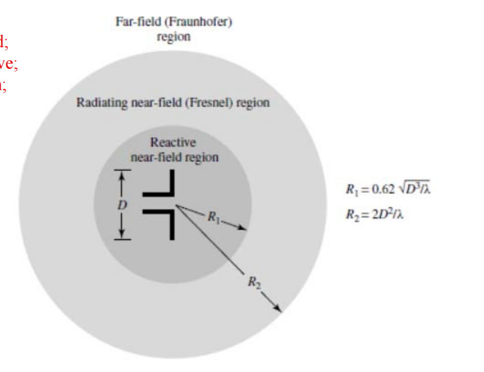
Field Zone

Near field: resonant, field;

Far field: propagation, wave;

Fresnel region: transition;

Antenna Parameters

• Radiation patterns
• Radiation Intensity
• Power Density
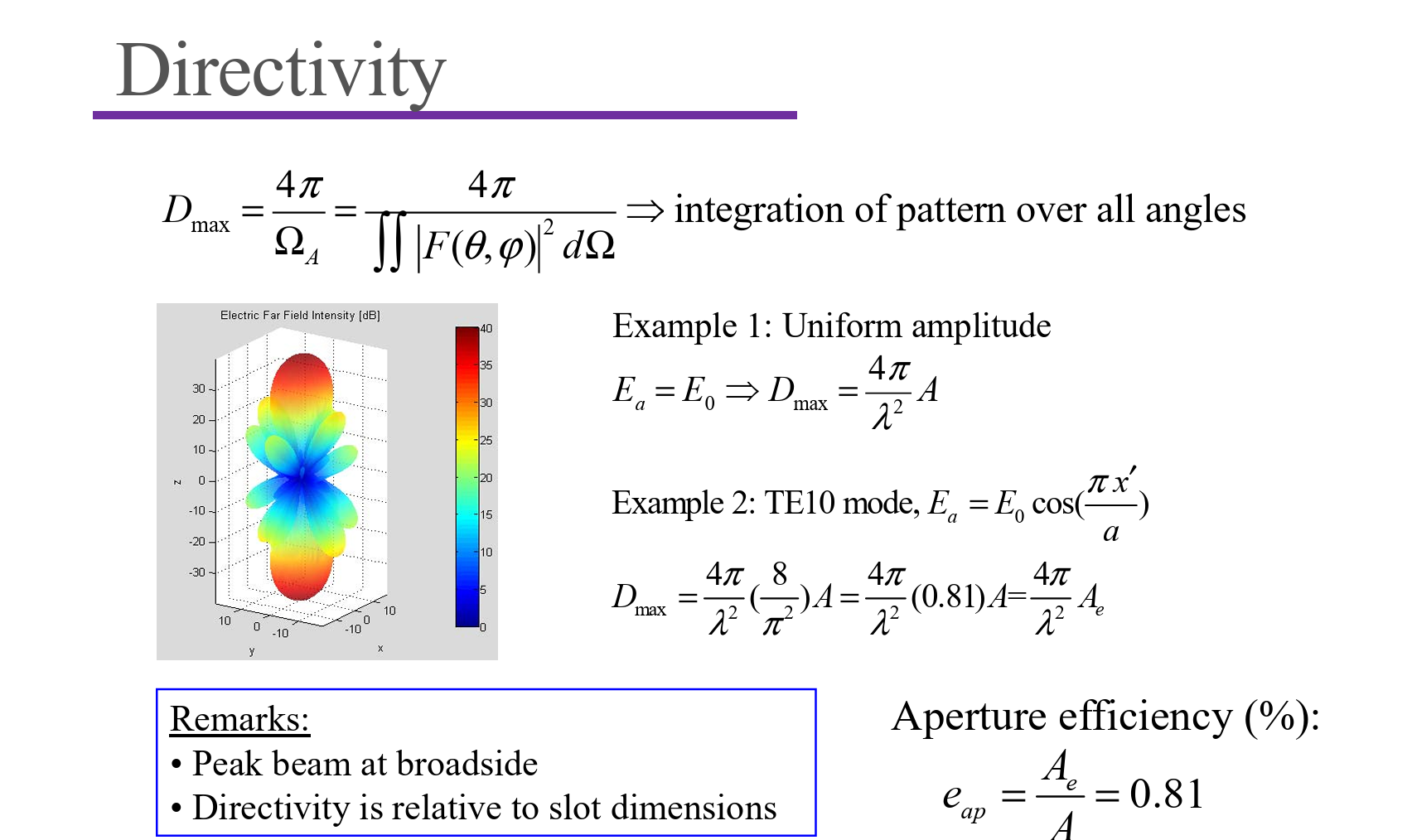
• Directivity (方向性) and Gain (重要！)
• Polarization
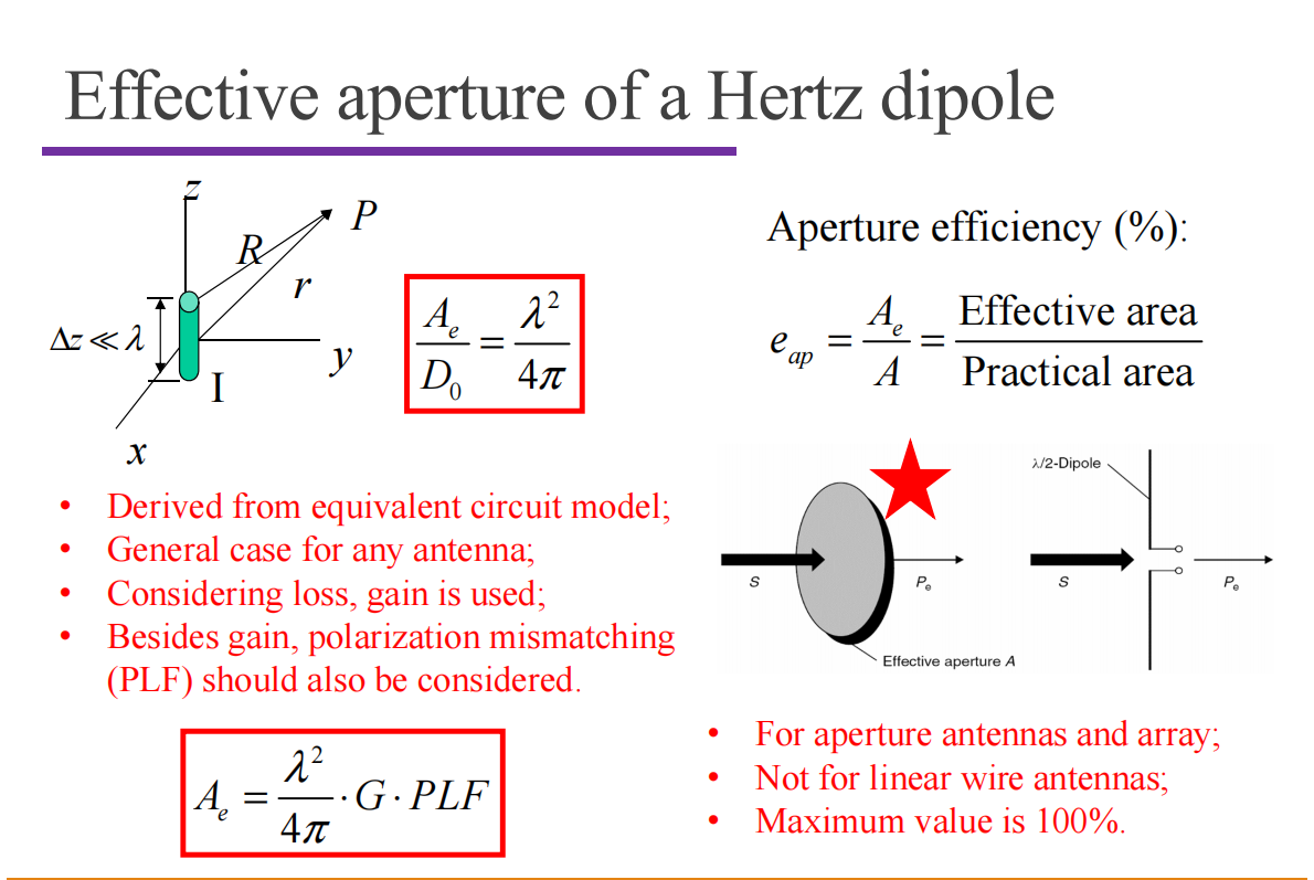
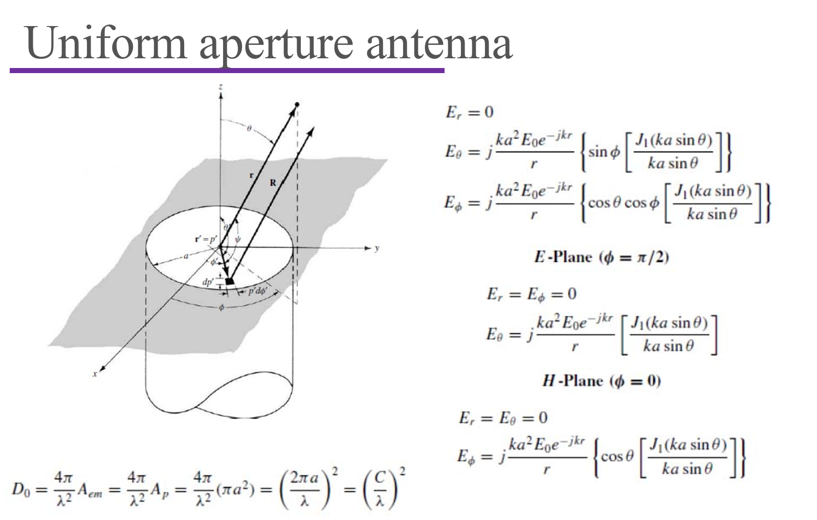
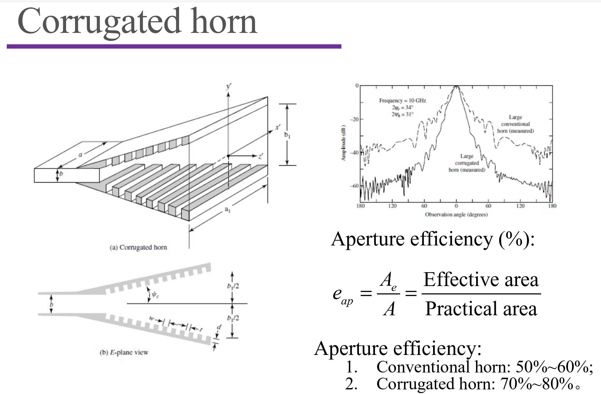
• Effective Aperture(等效口面) and Aperture efficienty(口面效率)

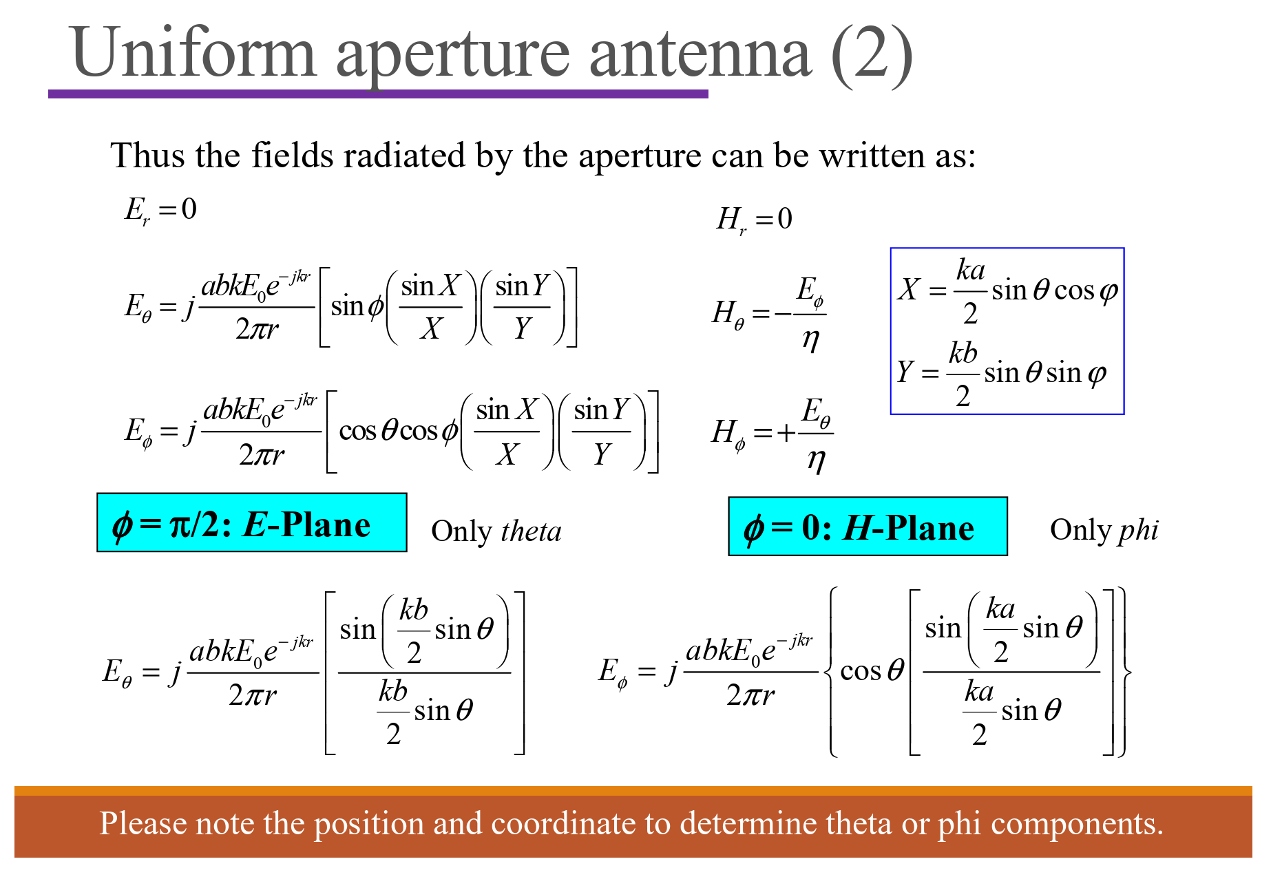
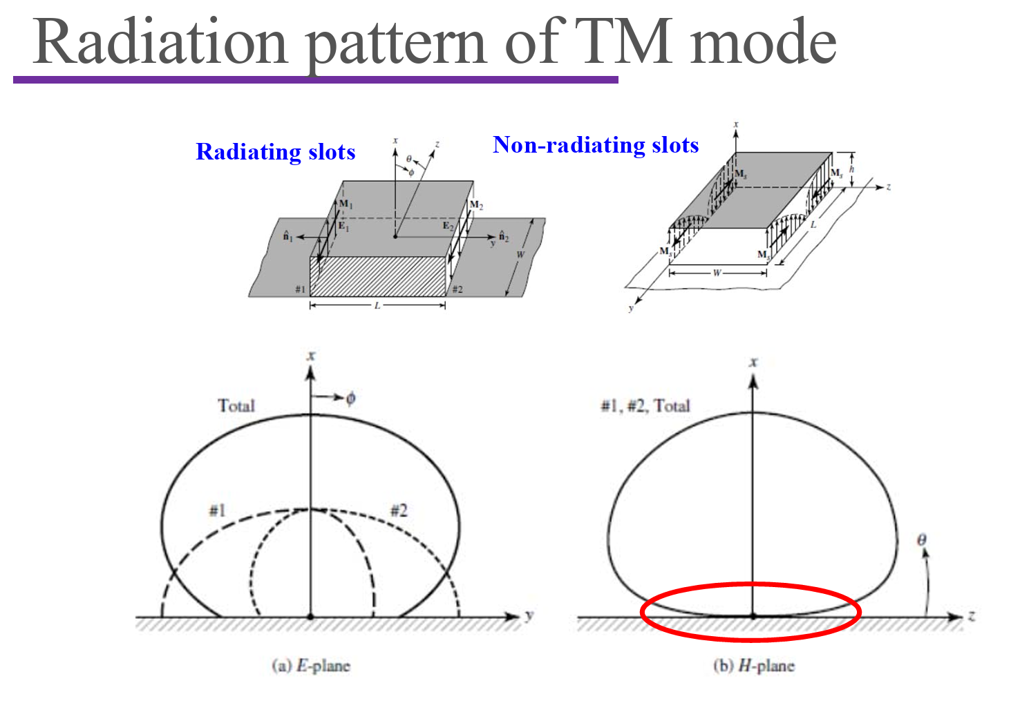
E 面：与电场方向平行的面

H 面：与磁场方向平行的面

Pattern Parameters

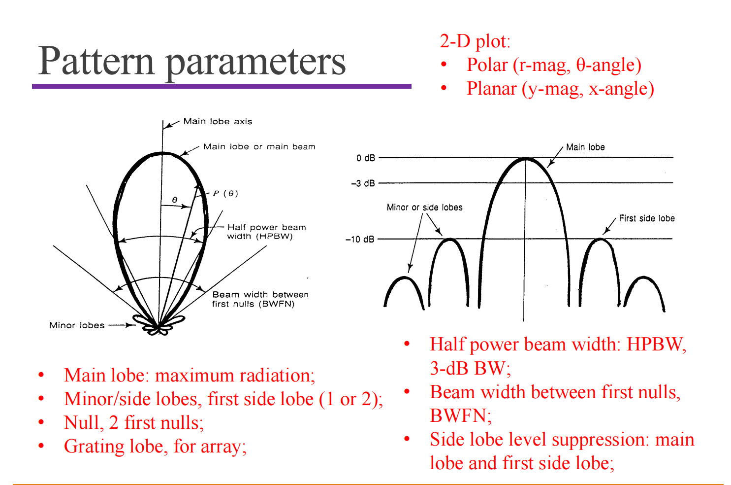
Often use log scale.

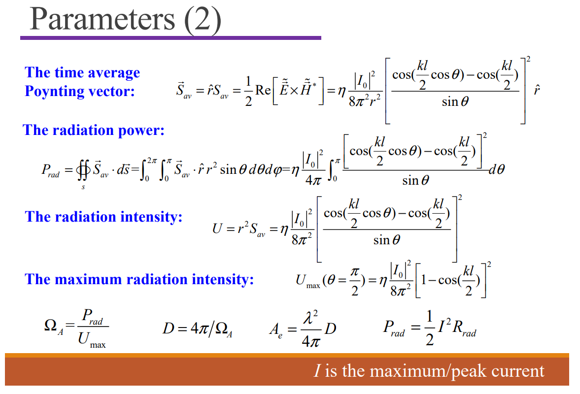
Power Density

Instantaneous Poynting vector $\vec S(x, y, z, t)$

Radiation Power Density = Time average Poynting vector $\vec S_{av}(x, y, z)=\frac1T\int_0^T\vec S(x, y, z, t)\mathrm dt = \frac12\text{Re}[\tilde{\vec E} \times \tilde{\vec H^*}]$

Total Radiation Power $P_{rad} = \oiint_S[\tilde{\vec E} \times \tilde{\vec H^*}] \cdot \mathrm d\vec s$

Radiation Intensity

$$ U(\theta, \varphi) = r^2 S(r, \theta, \varphi) $$

Isotropic 各向同性

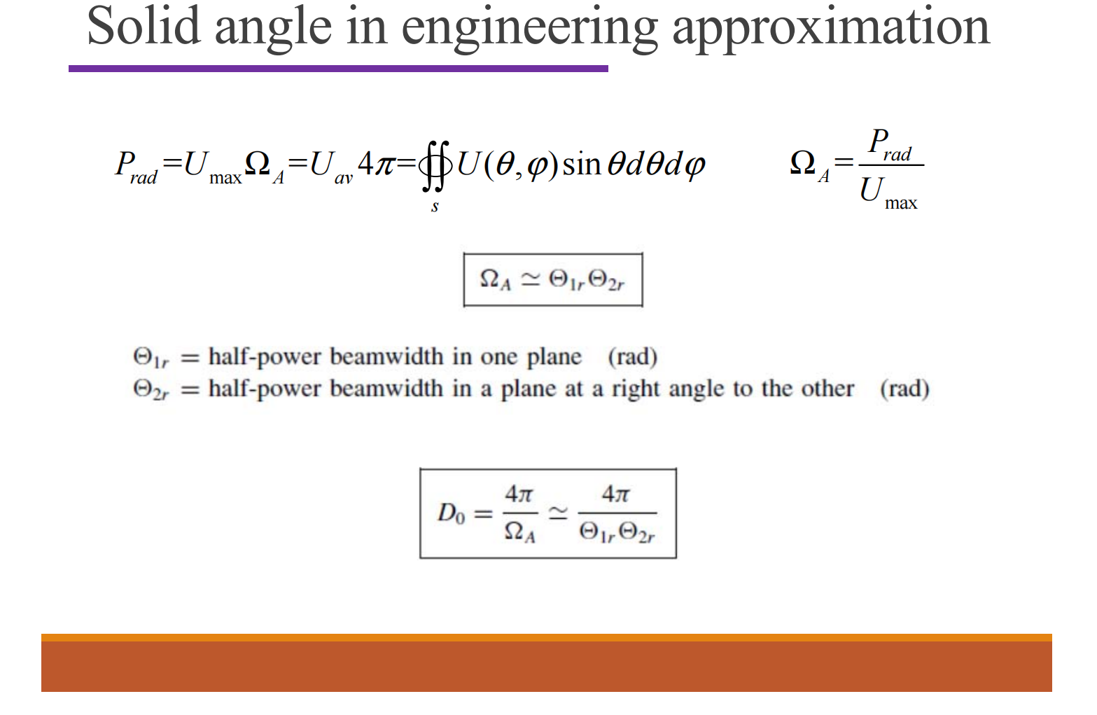
$$ P_{rad} = \int_{0}^{2\pi}\int_{0}^{\pi}U\sin\theta\mathrm d\theta\mathrm d\varphi $$

Directivity

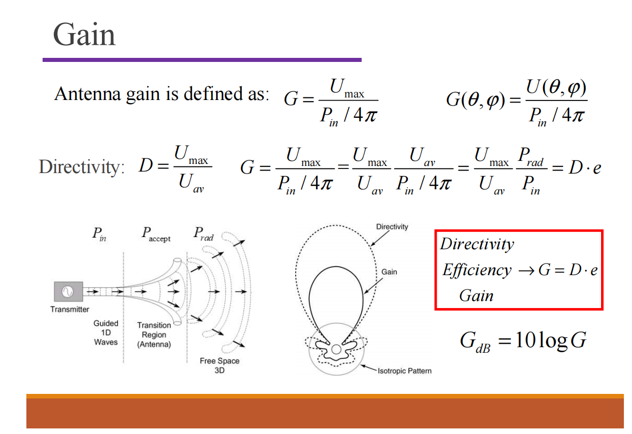
$$ D = \frac{U_{\max}}{U_{av}} = \frac{P_{\max}}{P_{rad}/4\pi} $$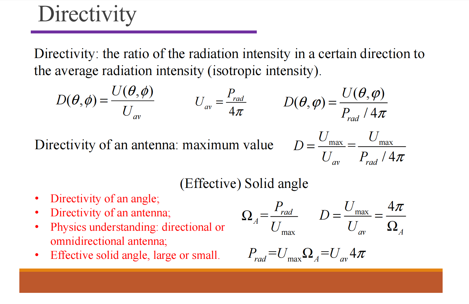

Gain

$$ G = \frac{U_{\max}}{P_{in}/4\pi} $$

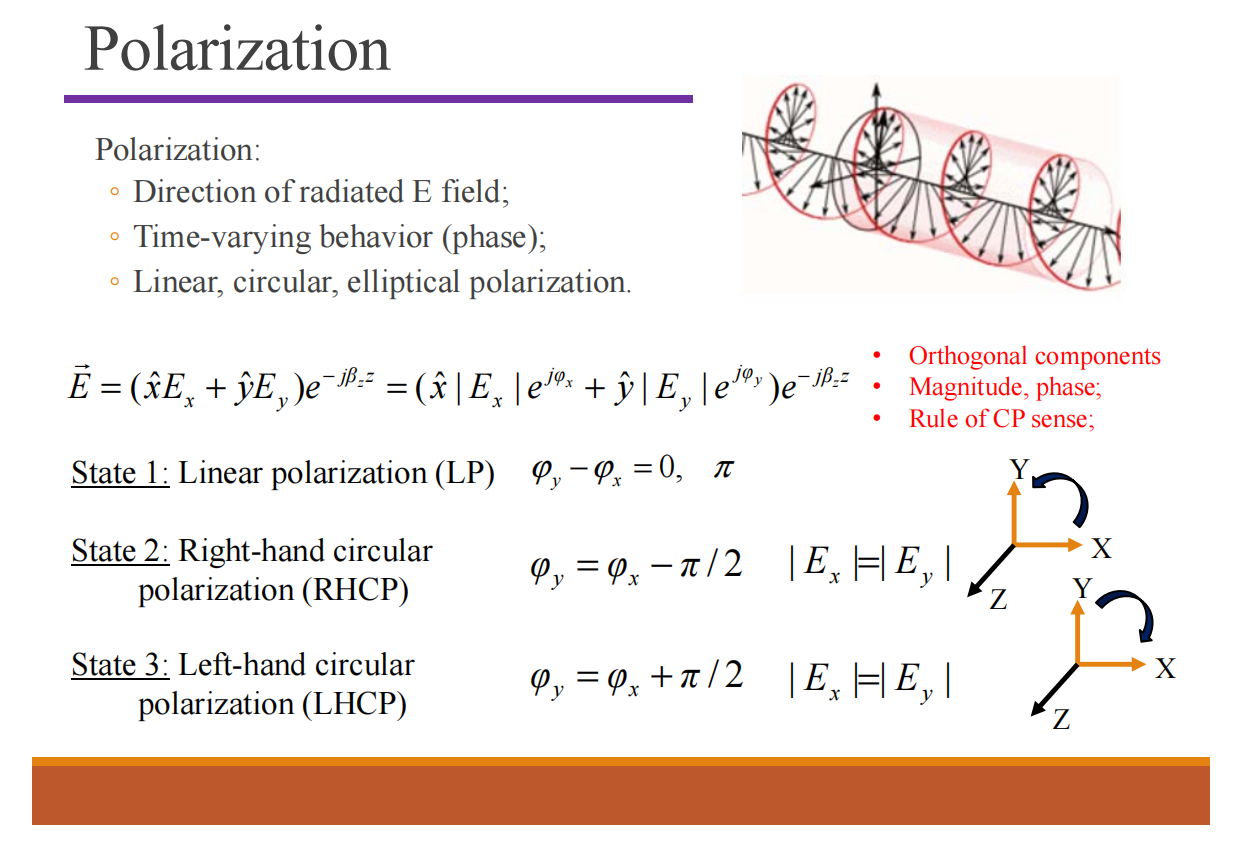
Polarization

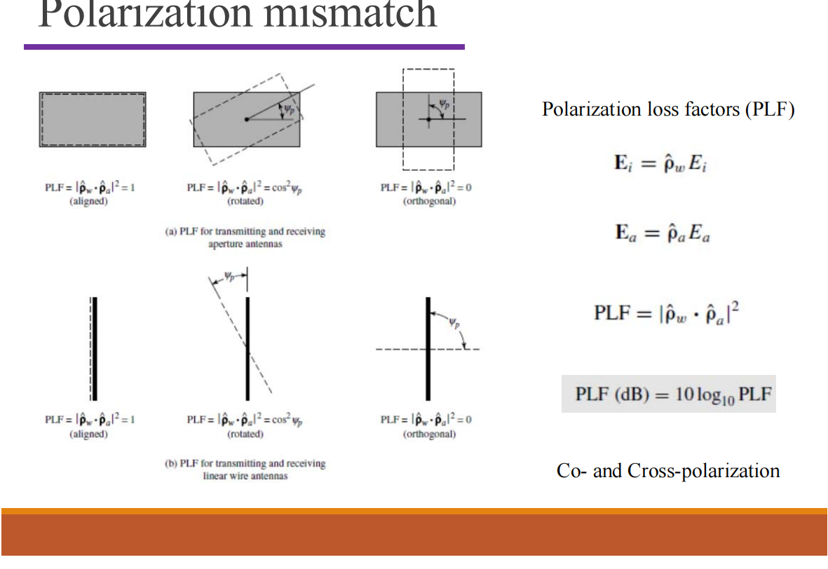
Polarization Mismatch:

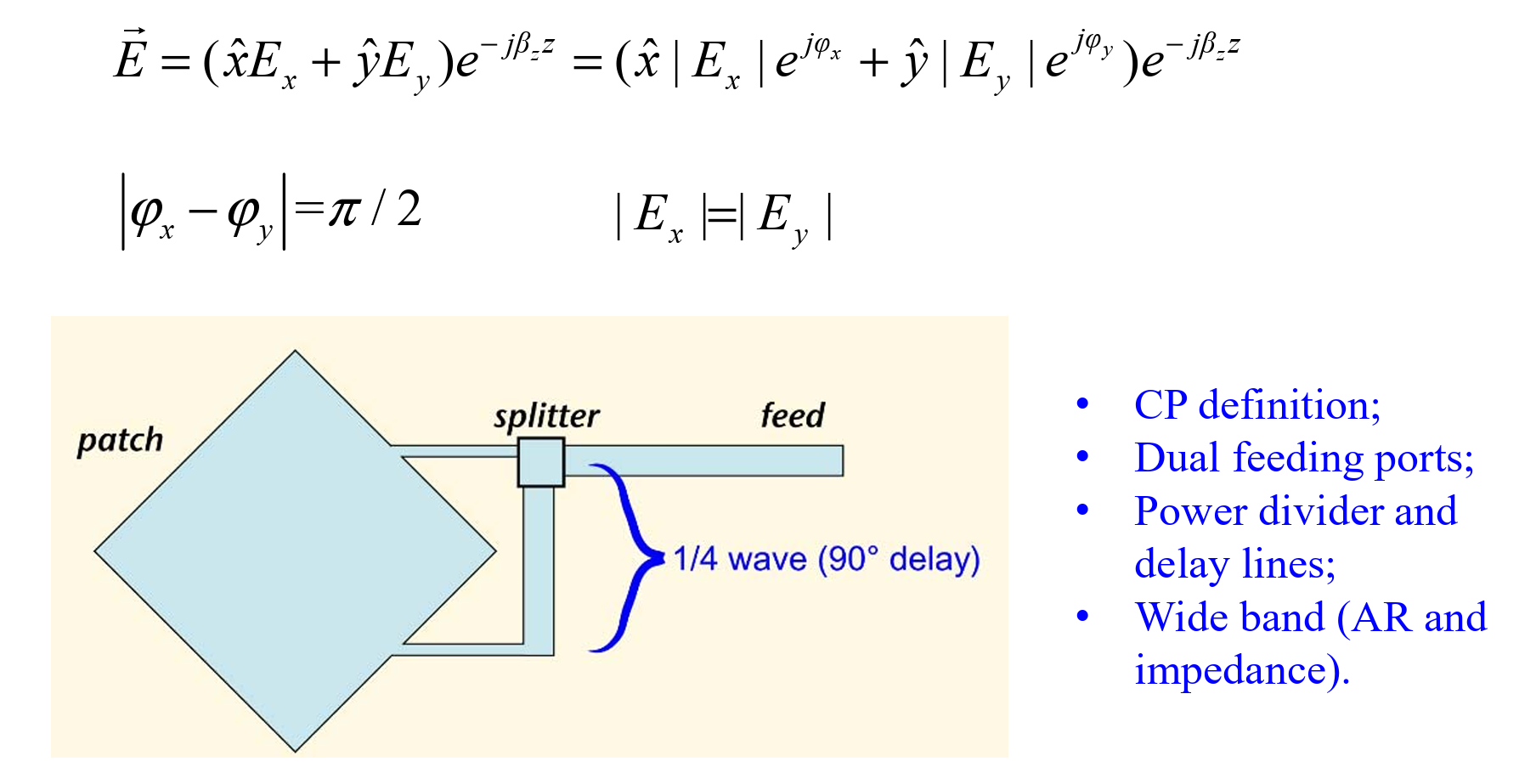
CP

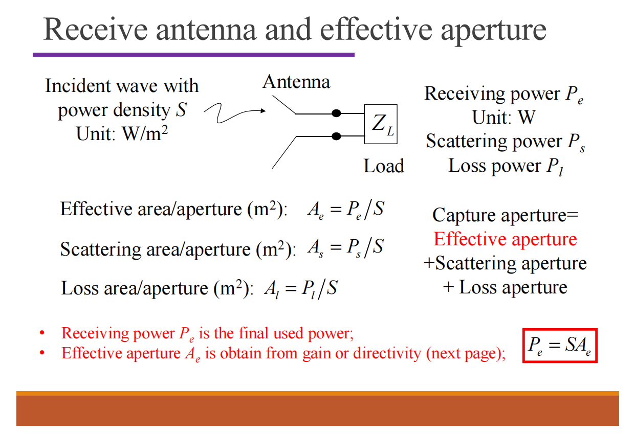
Effective Aperture and Aperture efficiency

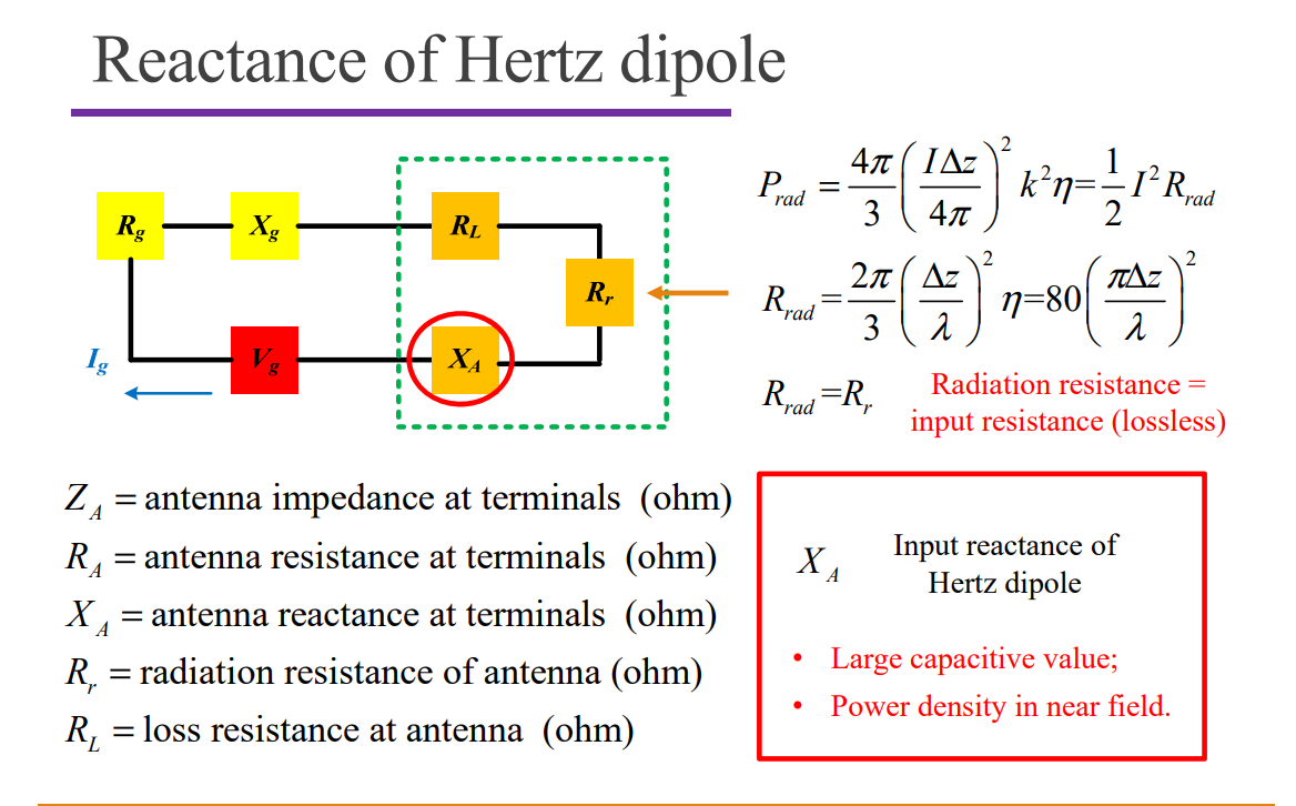
Circuit Parameters

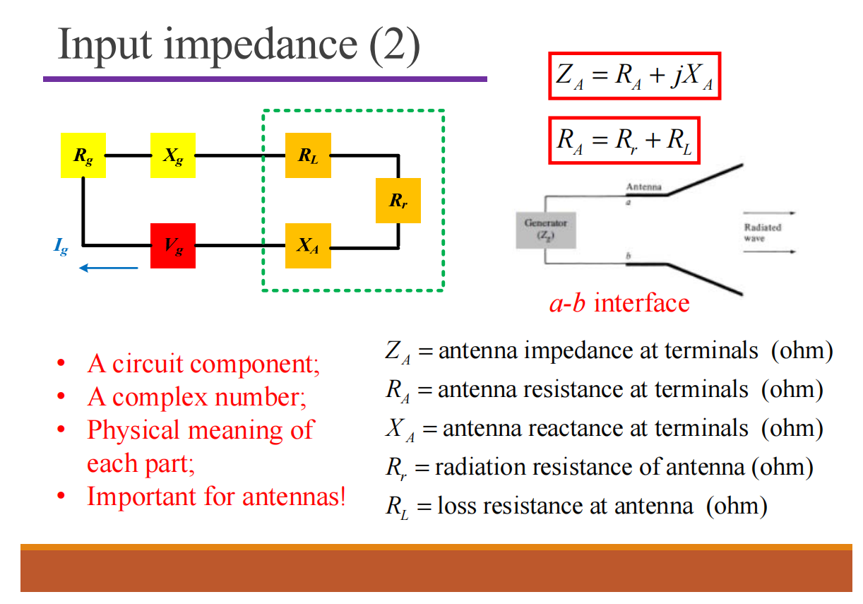
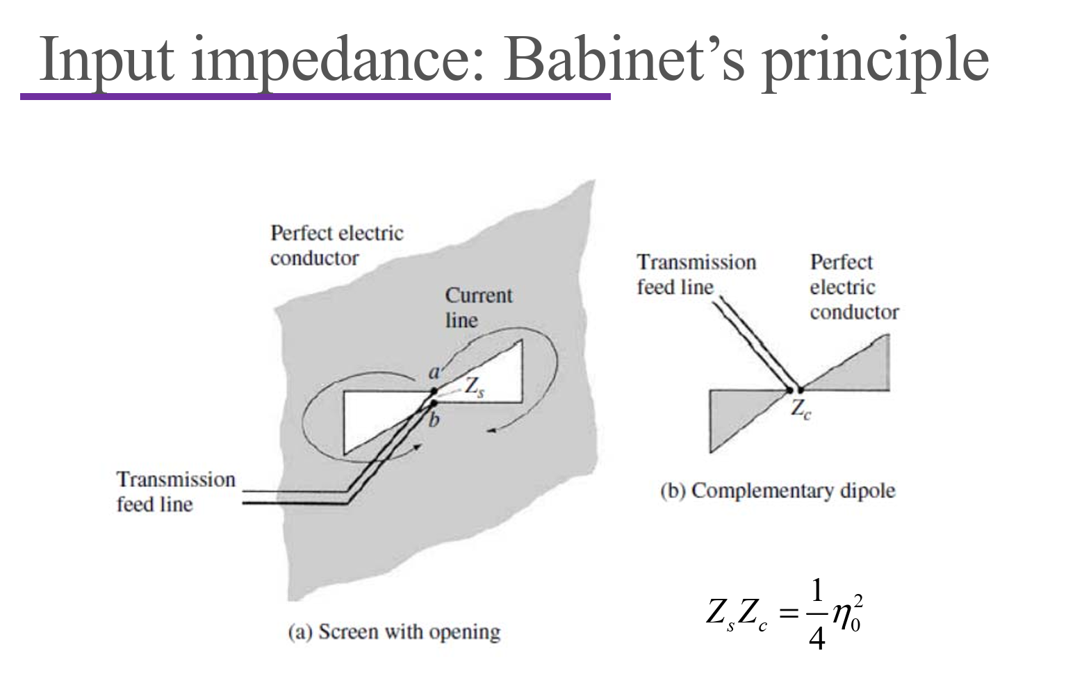
Input impedance

Input impedance definition:

• the impedance presented by an antenna at its terminals
• the ratio of the voltage to current at its terminals
• the ratio of the electric to magnetic fields at its terminals

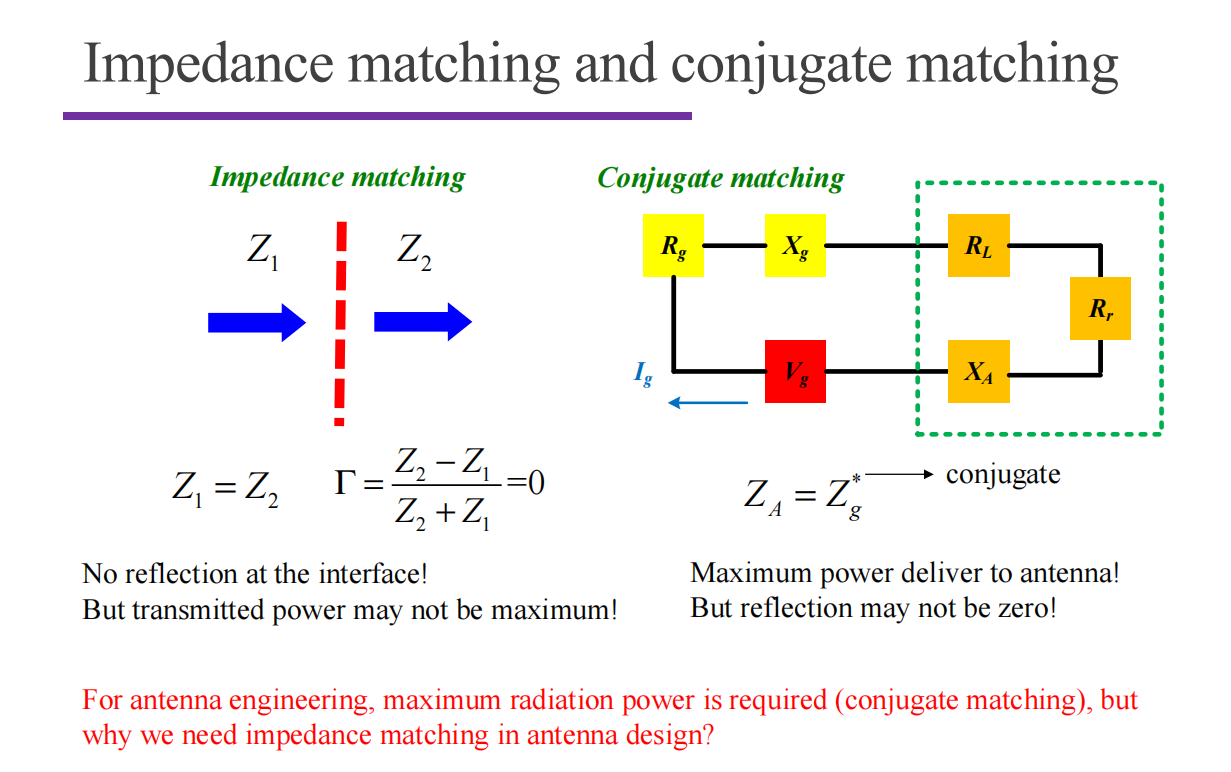
Conjugate Matching

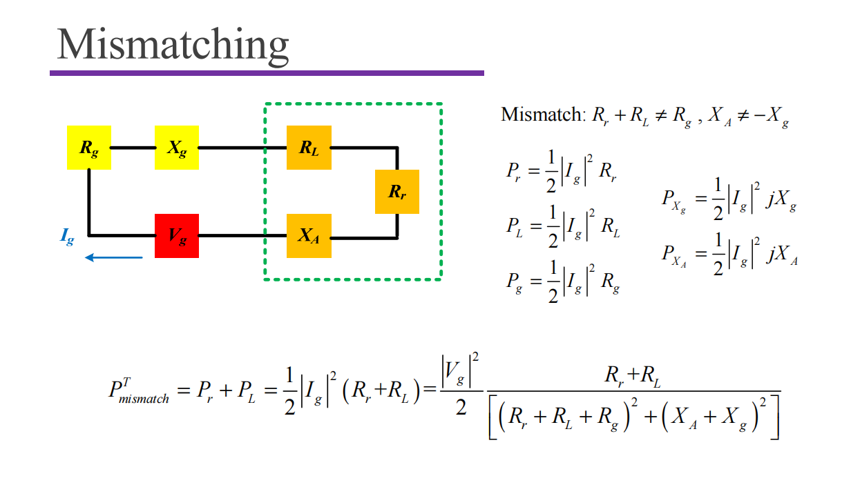
$$ Z_A = Z_g^* $$

Mismatching

Radiation Resistance

$$ P_{rad} = \frac12|I_g|^2R_r = \oiint_S\vec S_{av} \cdot \rm d\vec s $$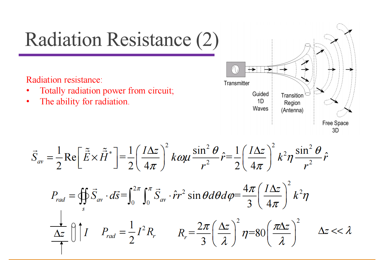

Scattering Parameters

$$ \frac{\Gamma^2}{Z_1} + \frac{T^2}{Z_2} = 1 $$

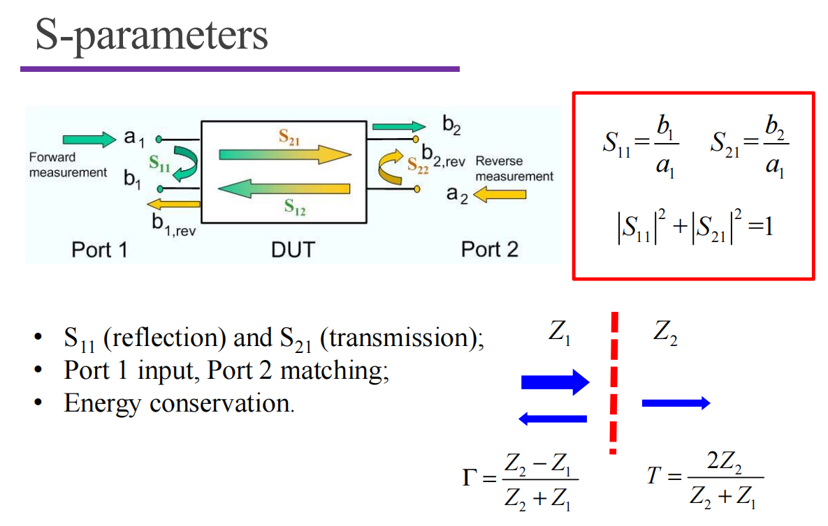
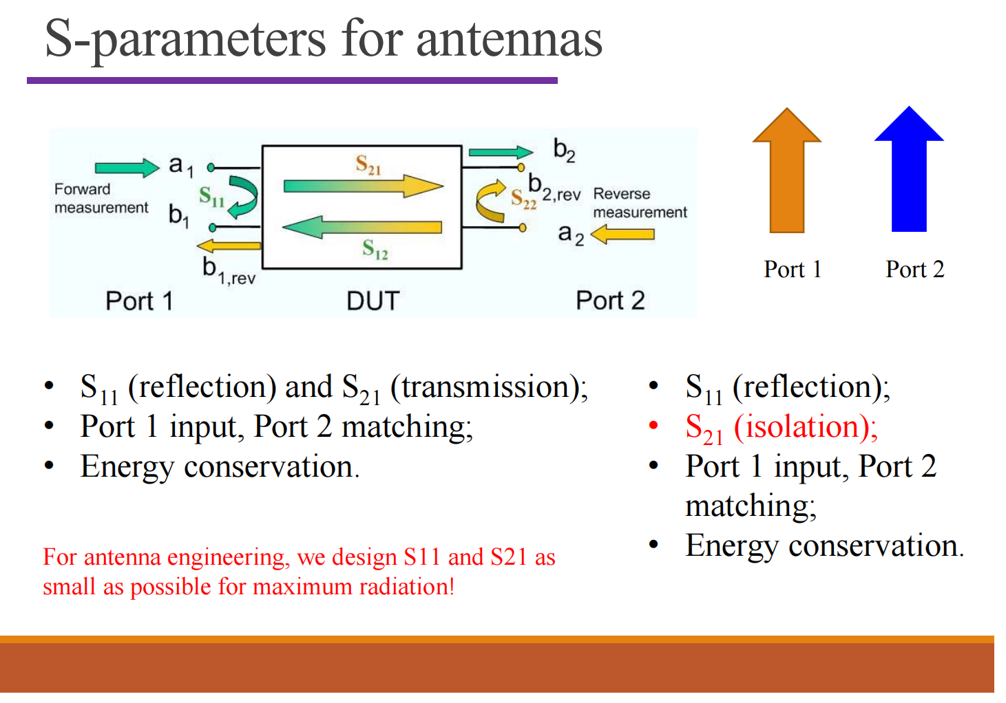
二端口网络通常用于描述二天线问题。 $S_{11}$ 表示天线1的反射， $S_{21}$ 表示天线1到天线2的耦合，均不利于信号的传播。我们希望让 $1 - S_{11}^2 - S_{21}^2$ 尽可能大。

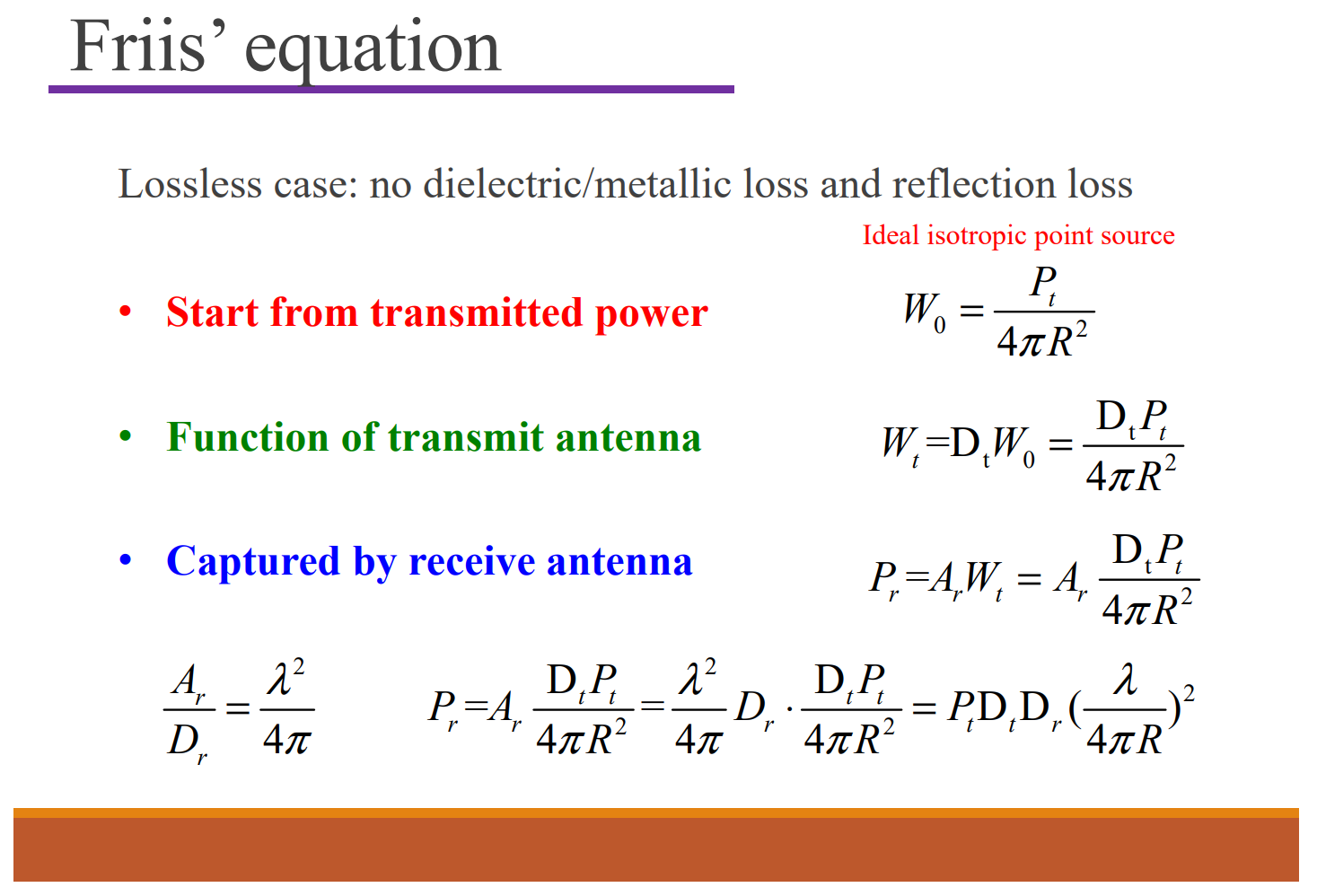
Link Calculation

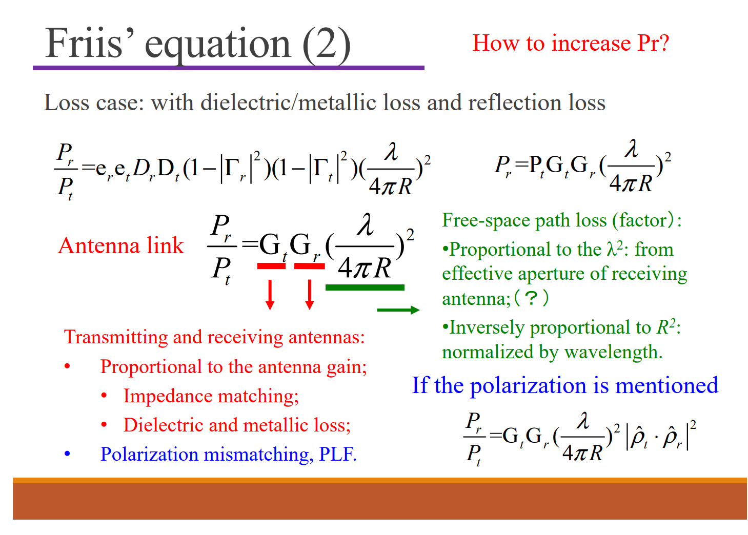
Friis’s Equation

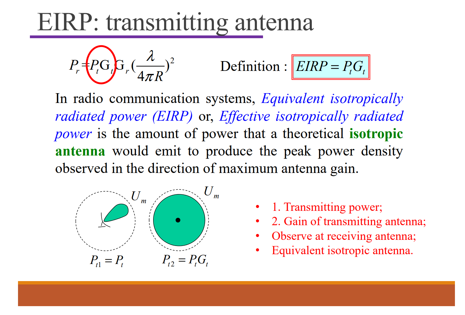
EIRP

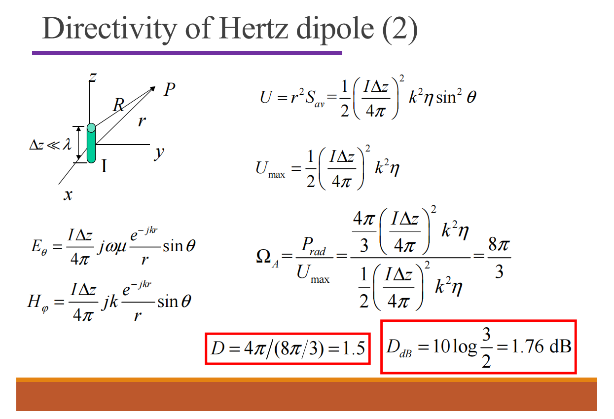
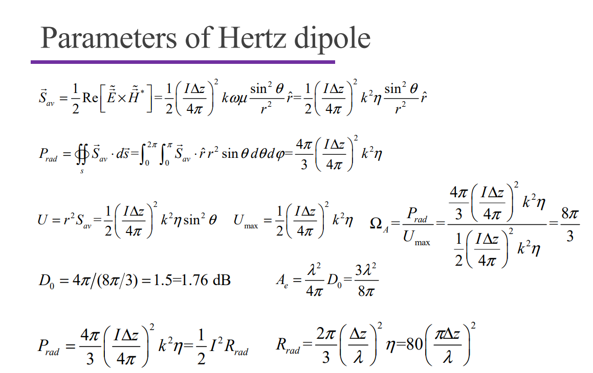
赫兹偶极子的辐射电阻： $80\pi^2(\frac{\Delta z}{\lambda})^2$ ，方向性 $\frac{2}{3}$ 。

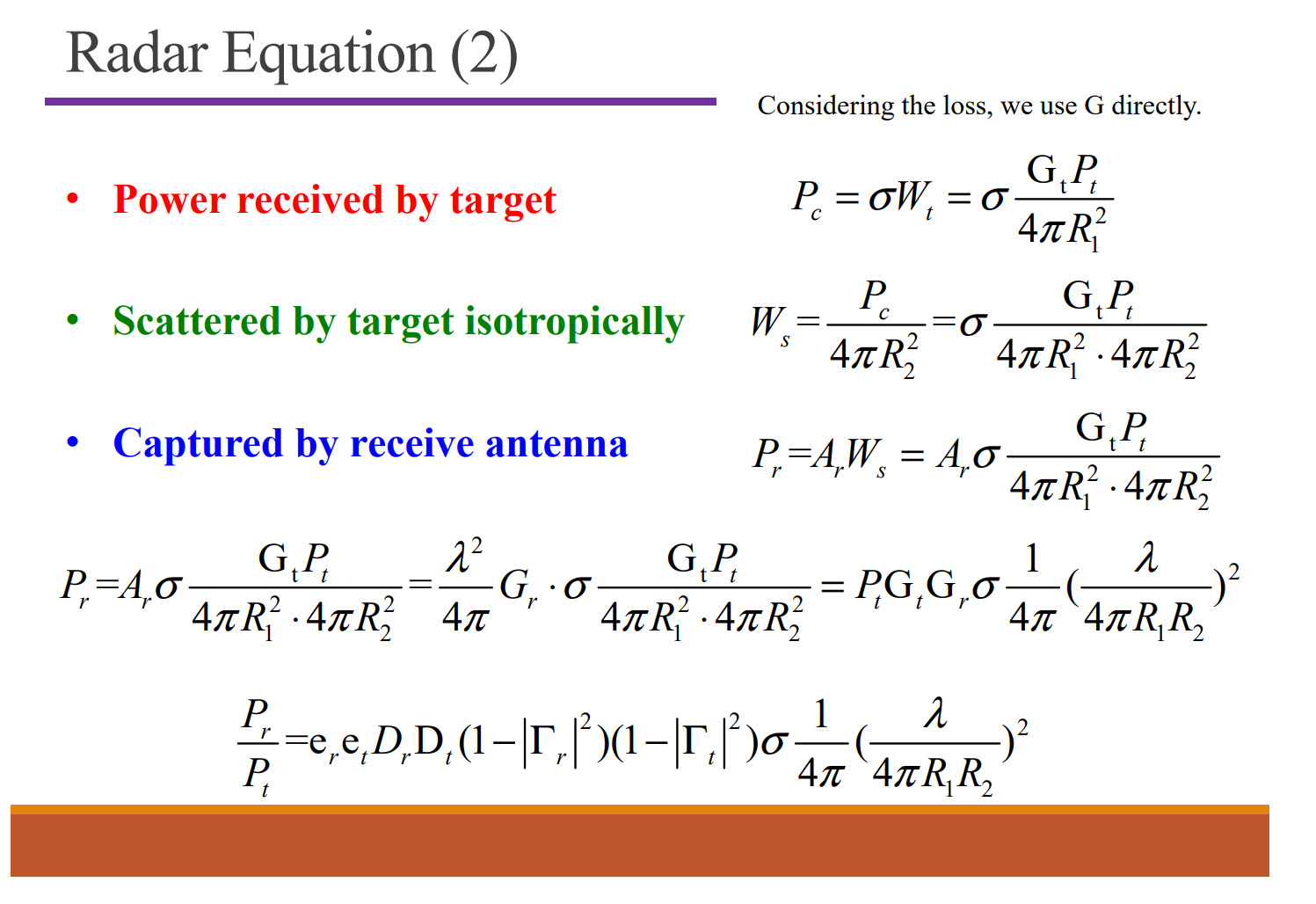
Radar Equation

RCS(Radar cross section)

RCS (σ) of a radar target is an effective area that intercepts the transmitted radar power and then
scatters that power isotropically back to the radar receiver.

$$ \sigma=\lim_{R\to\infty}\frac{W_{o}4\pi R^2}{W_i} $$

• $W_i$ , $W_o$ and $R$ are known;
• $\sigma$ converges.

Antenna Theorems

$$ \boxed{P_r=\mathrm{P}_t\mathrm{G}_t\mathrm{G}_r(\frac{\lambda}{4\pi R})^2} $$ $$ P_{r}=P_{t}\mathrm{e}_{r}\mathrm{e}_{t}D_{r}\mathrm{D}_{t}(1-\left|\Gamma_{r}\right|^{2})(1-\left|\Gamma_{t}\right|^{2})(\frac{\lambda}{4\pi R})^{2} $$

In radar:

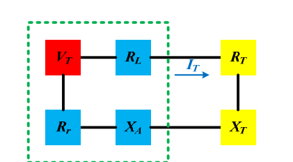
$$ P_{r}=P_{t}\mathrm{G}_{t}\mathrm{G}_{r}\sigma\frac{1}{4\pi}(\frac{\lambda}{4\pi R_{1}R_{2}})^{2} $$

Equivalent circuit model

$R_r$ ：接收天线反射会释放能量。

Duality Theorem

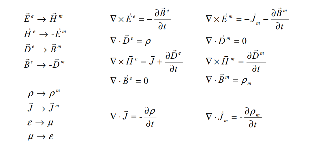
电 -> 磁，不变号；
磁 -> 电，变号。

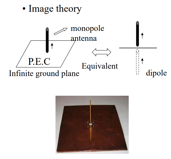
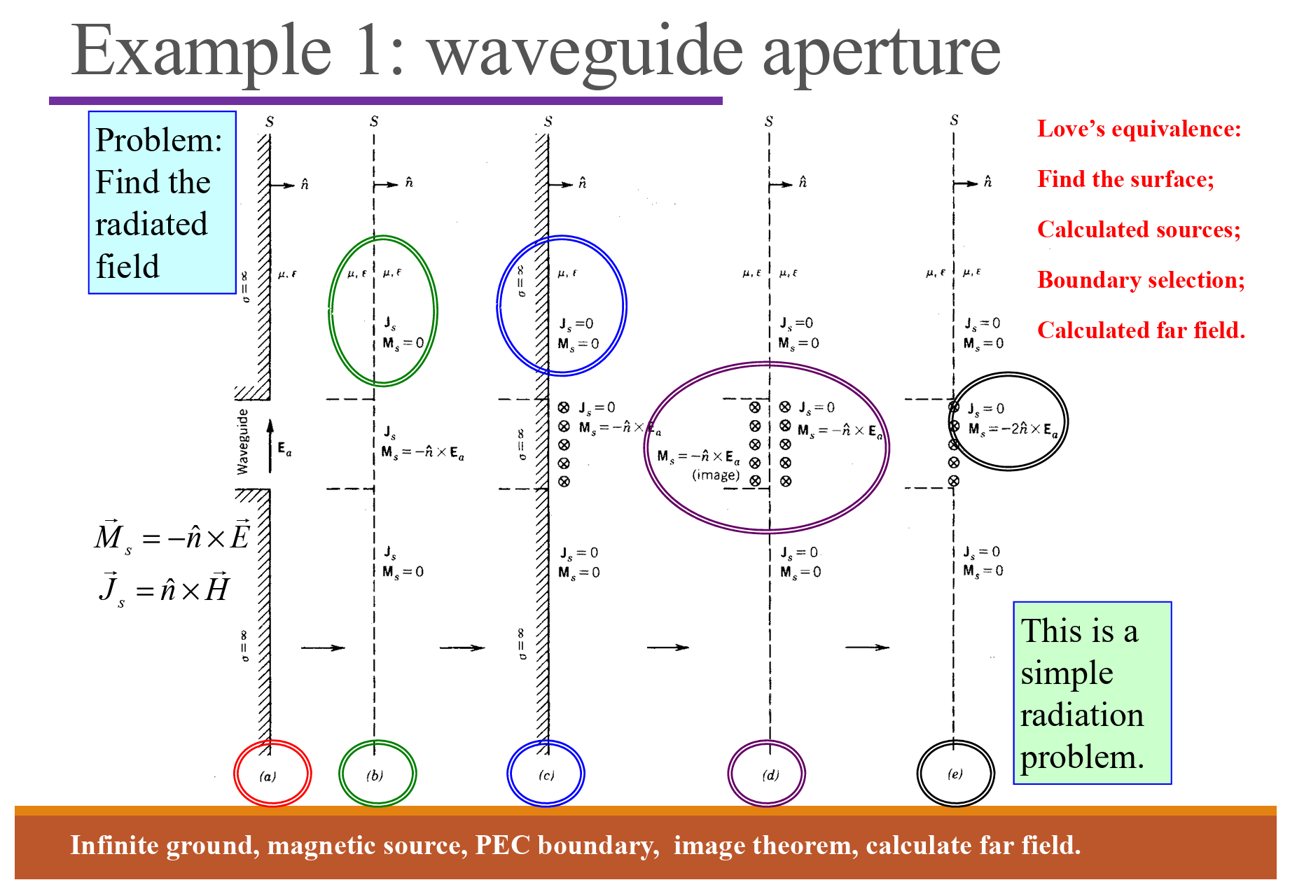
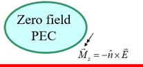
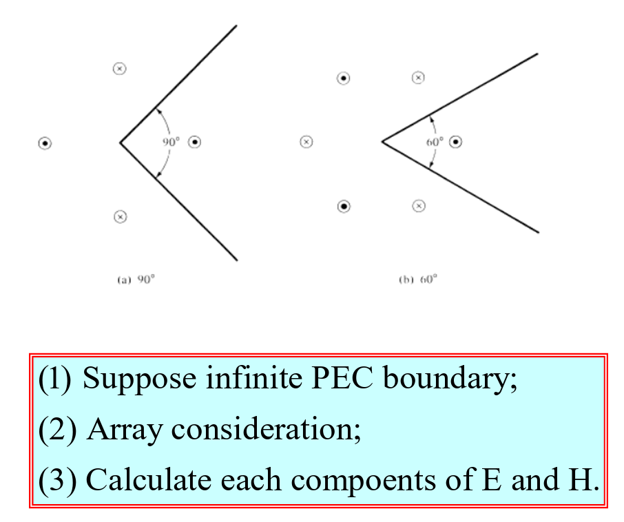
Image Theorem

PEC：完美电导体

PMC：完美磁导体

定理条件：

• PEC or PMC
• Infinite boundary

PEC

$$ \begin{aligned}&\hat{n}\times\vec{E}=0\\&\hat{n}\cdot\vec{B}=0\end{aligned} $$

PMC

$$ \begin{aligned}&\hat{n}\times\vec{H}=0\\&\hat{n}\cdot\vec{D}=0\end{aligned} $$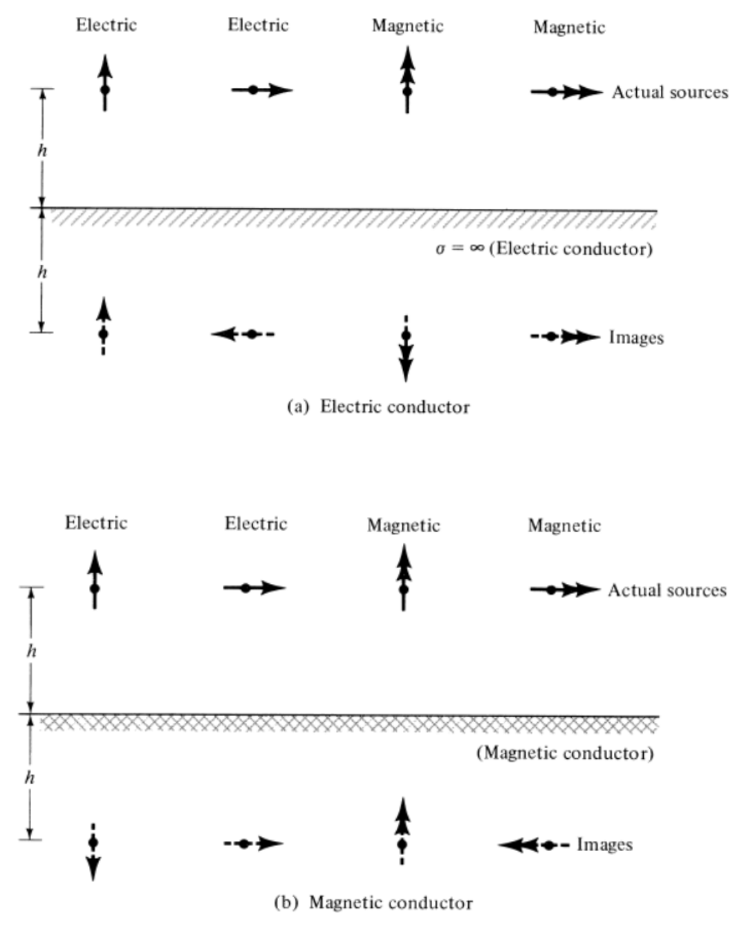

Note:

• Satisfied with boundary condition;
• Mirror source instead of PEC or PMC infinite boundary;
• Array: source and mirror source;
• Current loop: upper inside, lower outside.

Reciprocity Theorem

In radiation pattern,

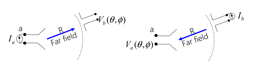
Transmitting pattern of antenna “a”

$$ Z_{_{ba}}(\theta,\varphi)=\frac{V_{_b}(\theta,\varphi)}{I_{_a}} $$

Receiving pattern of ante

$$ Z_{ab}(\theta,\varphi)=\frac{V_{a}(\theta,\varphi)}{I_{b}} $$

Then,

$$ Z_{ab}(\theta,\phi)=Z_{ba}(\theta,\phi) $$

Lorentz Reciprocity Theorem

$$ -\nabla\cdot(\vec{E}_{1}\times\vec{H}_{2}-\vec{E}_{2}\times\vec{H}_{1})=\vec{E}_{1}\cdot\vec{J}_{2}+\vec{H}_{2}\cdot\vec{M}_{1}-\vec{E}_{2}\cdot\vec{J}_{1}-\vec H_1 \cdot \vec M_2\\ -\oiint_{S}(\vec{E}_{1}\times\vec{H}_{2}-\vec{E}_{2}\times\vec{H}_{1})\cdot ds^{'}=\iiint_{V}\left(\vec{E}_{1}\cdot\vec{J}_{2}+\vec{H}_{2}\cdot\vec{M}_{1}-\vec{E}_{2}\cdot\vec{J}_{1}-\vec H_1 \cdot \vec M_2\right)dv^{'} $$

Far field:

$$ \vec{H}_i=\hat{r}\times\vec{E}_i/\eta;\quad d\vec{s}=\hat{n}ds=\hat{r}ds $$ $$ (\vec{E}_1\times\vec{H}_2-\vec{E}_2\times\vec{H}_1)\cdot\hat{r}=(\hat{r}\times\vec{E}_1)\cdot\vec{H}_2-(\hat{r}\times\vec{E}_2)\cdot\vec{H}_1=0 $$ $$ \iiint_{V}\Big(\vec{E}_{1}\cdot\vec{J}_{2}+\vec{H}_{2}\cdot\vec{M}_{1}-\vec{E}_{2}\cdot\vec{J}_{1}-\vec{H}_{1}\cdot\vec{M}_{2}\Big)d\nu^{'}=0\\\iiint_{V}\Big(\vec{E}_{1}\cdot\vec{J}_{2}-\vec{H}_{1}\cdot\vec{M}_{2}\Big)d\nu^{'}=\iiint_{V}\Big(\vec{E}_{2}\cdot\vec{J}_{1}-\vec{H}_{2}\cdot\vec{M}_{1}\Big)d\nu^{'} $$

Reaction: Reciprocity theorem: $\langle 1 2\rangle=\langle 2,1\rangle$

$$ \left\langle1,2\right\rangle=\int_{V}(\vec{E}_{1}\cdot\vec{J}_{2}-\vec{H}_{1}\cdot\vec{M}_{2})d\nu\quad\left\langle2,1\right\rangle=\int_{V}(\vec{E}_{2}\cdot\vec{J}_{1}-\vec{H}_{2}\cdot\vec{M}_{1})d\nu $$

If only current-source

$$ \iiint_V\vec{E}_1\cdot\vec{J}_2d\nu=\iiint_V\vec{E}_2\cdot\vec{J}_1d\nu\\ \vec{E}_1\cdot\vec{J}_2=\vec{E_2} \cdot \vec{J_1} $$

Non-reciprocity

Electron plasma (non-reciprocal media)

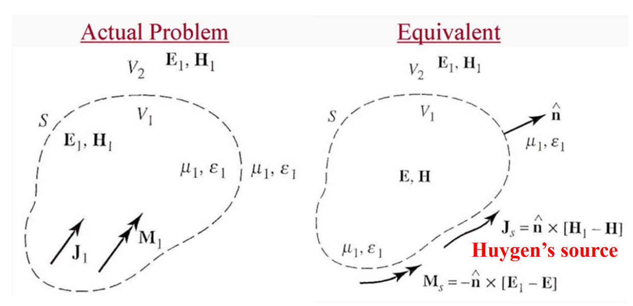
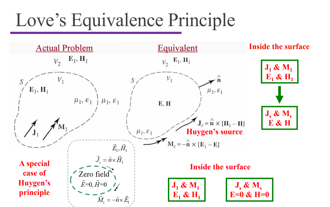
$$ \varepsilon = \begin{bmatrix}\varepsilon_{xx}&+ig&0\\-ig&\varepsilon_{yy}&0\\0&0&\varepsilon_{zz}\end{bmatrix} $$

Huygen’s Principle

Dipole Antenna

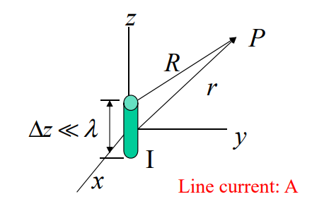
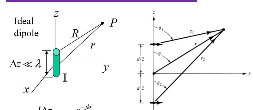
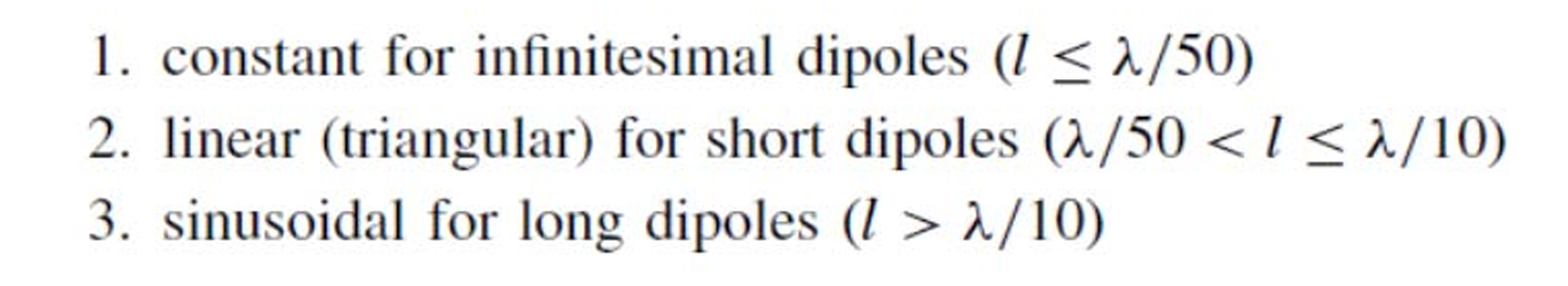
Hertz Dipole

• Infinite short length;
• Uniform distribution;
• Infinite small radius;

$$ E_\theta=\frac{I\Delta z}{4\pi}j\omega\mu\frac{e^{-jkr}}r\sin\theta \\ H_\varphi=\frac{I\Delta z}{4\pi}jk\frac{e^{-jkr}}r{\sin\theta}\\ \frac{E_\theta}{H_\varphi}=\sqrt{\frac{\mu_0}{\varepsilon_0}}=\eta $$

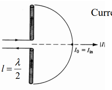
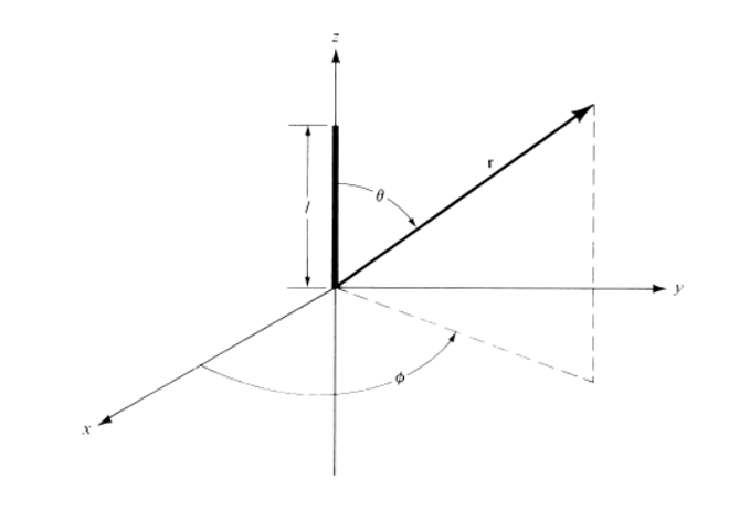
Finite Length Dipole

$$ I=\begin{cases}I_0\sin[k(\dfrac{l}{2}-z')]&0\leq z'\leq\dfrac{l}{2}\\ I_0\sin[k(\dfrac{l}{2}+z')]&-\dfrac{l}{2}\leq z'\leq0\end{cases} $$ $$ \vec{A}(x,y,z)=A_z\hat{z}=\hat{z}\int_{-l/2}^{l/2}\mu I(z’)\frac{e^{-j\kappa\Lambda}}{4\pi R}dz’\\R=\sqrt{\left(x-x’\right)^2+\left(y-y’\right)^2+\left(z-z’\right)^2} $$ $$ \begin{aligned}&\text{For phase:}&&R\cong r-z'\cos\theta\\&\text{For amplitude:}&&R\cong r\end{aligned} $$

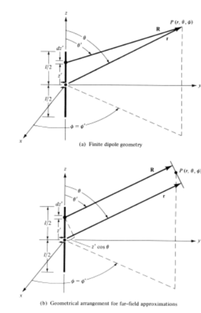
R is the distance between observer and source,
r is the distance between observer and origin.

Small Dipole

$$ \begin{aligned}&I(z’)\cong I_{in}(1-2|z’|/l)\\&\vec{A}(x,y,z)=A_z\hat{z}=\hat{z}\int_{-l/2}^{l/2}\mu I(z’)\frac{e^{-jkr}}{4\pi r}dz’\end{aligned} $$

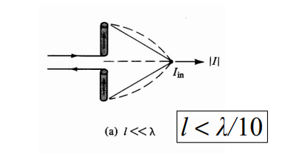
Then

$$ \vec{A}(x,y,z)=\hat{z}\mu\frac{e^{-jkr}}{4\pi r}\cdot\frac12I_{in}l\\ \vec{A}(\theta,r)=\frac12I_{in}l\mu\frac{e^{-jkr}}{4\pi r}(-\sin\theta\hat{\theta}+\cos\theta\hat{r}) $$ $$ \vec{E}=j\omega\mu I_{in}l\frac{e^{-jkr}}{8\pi r}\sin\theta\hat{\theta}\\\vec{H}=j\beta I_{in}l\frac{e^{-jkr}}{8\pi r}\sin\theta\hat{\varphi} $$

Note: half of the ideal infinitesima(Hertz) dipole

$$ \mathrm{Directivity}:\quad D=\frac{4\pi}{\Omega_A}\Rightarrow D_{\underset{dipole}{\operatorname*{small}}}=1.5 $$ $$ R_{rad}=20\left(\frac{\pi\Delta z}\lambda\right)^2=\frac14R_{rad}^\textit{Hertz dipole} $$ $$ P_{rad}=\frac14\frac{4\pi}3{\left(\frac{I\Delta z}{4\pi}\right)}^2k^2\eta{=}\frac12I^2R_{rad} $$

General Case

$$ E_{\theta}=j\eta\frac{I_0e^{-jkr}}{2\pi r}\Bigg[\frac{\cos(\frac{kl}2\cos\theta)-\cos(\frac{kl}2)}{\sin\theta}\Bigg]\\H_{\varphi}=j\frac{I_0e^{-jkr}}{2\pi r}\Bigg[\frac{\cos(\frac{kl}2\cos\theta)-\cos(\frac{kl}2)}{\sin\theta}\Bigg] $$

Beam width: change with length.

$$ \begin{aligned} &\textbf{The time average Poynting vector:}\\ &\vec{S}_{a\nu}=\hat{r}S_{a\nu}=\frac{1}{2}\mathrm{Re}\bigg[\tilde{\vec{E}}\times\tilde{\vec{H}}^{*}\bigg]=\eta\frac{\big|I_{0}\big|^{2}}{8\pi^{2}r^{2}}\bigg[\frac{\cos(\frac{kl}{2}\cos\theta)-\cos(\frac{kl}{2})}{\sin\theta}\bigg]^{2}\hat{r} \\ &P_{rad}=\oint_{s}\vec{S}_{a\nu}\cdot d\vec{s}=\int_{0}^{2\pi}\int_{0}^{\pi}\vec{S}_{a\nu}\cdot\vec{r}r^{2}\sin\theta d\theta d\varphi=\eta\frac{\left|I_{0}\right|^{2}}{4\pi}\int_{0}^{\pi}\frac{\left[\cos(\frac{kl}{2}\cos\theta)-\cos(\frac{kl}{2})\right]^{2}}{\sin\theta}d\theta \\ &\begin{aligned}&\text{The radiation intensity:}\\&&U=r^2S_{av}=\eta\frac{\left|I_0\right|^2}{8\pi^2}\left[\frac{\cos(\frac{kl}2\cos\theta)-\cos(\frac{kl}2)}{\sin\theta}\right]^2\\&&=\frac{\pi}{2}=\frac{\left|I_{0}\right|^{2}}{2}=\frac{k_{0}}{2}=\frac{k_{0}}{2}\end{aligned}& \begin{matrix}{l}\\\end{matrix}) \\ &\Omega_A=\frac{P_{rad}}{U_{\max}}\quad D=4\pi/\Omega_A\quad A_e=\frac{\lambda^2}{4\pi}D\quad P_{rad}=\frac12I^2R_{rad} \end{aligned} $$

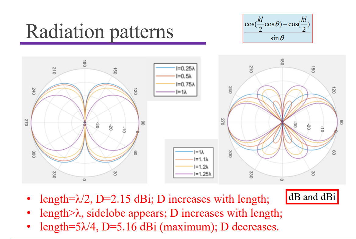
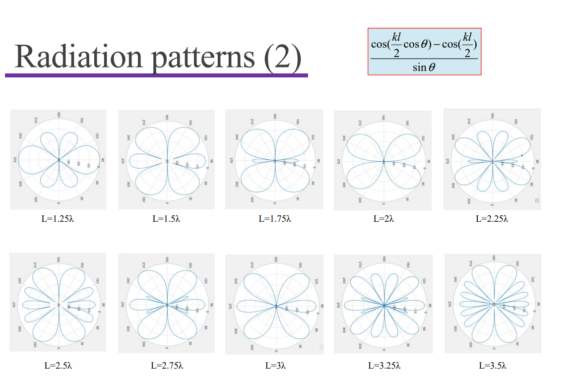
Input Impedance

Input resistance $R_r$ :

• calculated by E and H at port;
• take the real part (lossless).

Radiation resistance $R_{rad}$ :

• calculated by E and H at far-field;

$$ P_{rad}=\frac12{\left|I\right|}^2R_{rad}\quad P_{rad}=\frac12{\left|I_{in}\right|}^2R_r $$

I is the maximum/peak current.

General Relation:

$$ R_r=R_{rad}/\sin^2\left(\frac{kl}2\right) $$

Half-wavelength dipole

$$ I(z)=I_0\sin(\frac\pi2-k\left|z\right|) $$ $$ E_\theta(r,\theta,\varphi)=j\eta I_0\frac{e^{-jkr}}{2\pi r}\frac{\cos(\frac\pi2\cos\theta)}{\sin\theta}\\H_\varphi(r,\theta,\varphi)=jI_0\frac{e^{-jkr}}{2\pi r}\frac{\cos(\frac\pi2\cos\theta)}{\sin\theta} $$ $$ \vec{S}_{a\nu}=\hat{r}S_{a\nu}=\frac{1}{2}\operatorname{Re}\bigg[\tilde{\vec{E}}\times\tilde{\vec{H}}^{*}\bigg]=\eta\frac{\big|I_{0}\big|^{2}}{8\pi^{2}r^{2}}\bigg[\frac{\cos(\frac{\pi}{2}\cos\theta)}{\sin\theta}\bigg]^{2}\hat{r}\\ P_{rad}=\oint_sS_{a\nu}\cdot d\vec{s}=\int_0^{2\pi}\int_0^\pi\vec{S}_{a\nu}\cdot\hat{r}r^2\sin\theta d\theta d\varphi=\eta\frac{\left|I_0\right|^2}{4\pi}\int_0^\pi\frac{\cos^2(\frac\pi2\cos\theta)}{\sin\theta}d\theta $$ $$ D=4\pi/\Omega_{A}=1.643=2.15\mathrm{dBi}\\ A_e=\frac{\lambda^2}{4\pi}D_0\cong0.13\lambda^2 $$

Edge capacitive effect:

• Terminal (open-end)
  current is not ideal zero;
• Effective length is longer

$$ R_r=R_{rad}=\frac{2P_{rad}}{\left|I_0\right|^2}\cong73\left(\Omega\right)\\ Z_A=73+j43\left(\Omega\right) $$

Applications

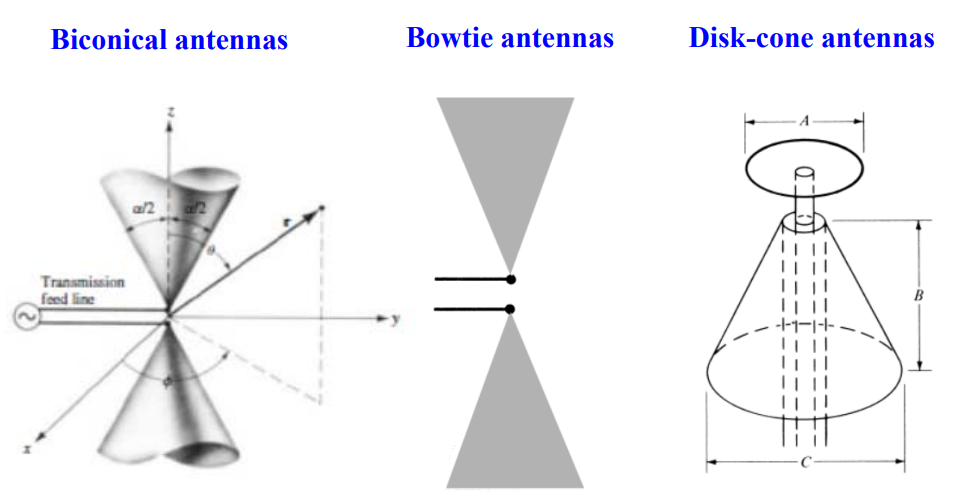
Wideband Antennas

Folded Dipole

$$ Z_{{folded}}=4Z_A $$

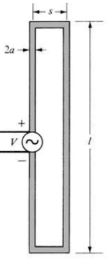
Increase Input Impedance

Log-periodic & Yagi-Uda antenna

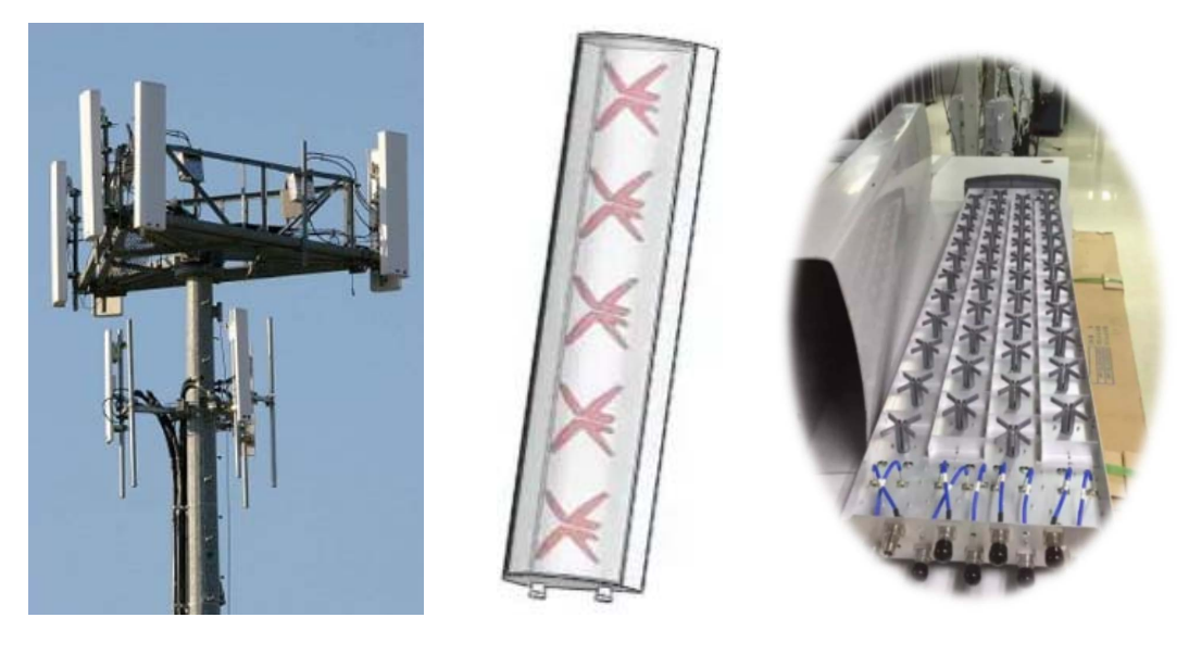
Dipole Antennas in base station

Monopole

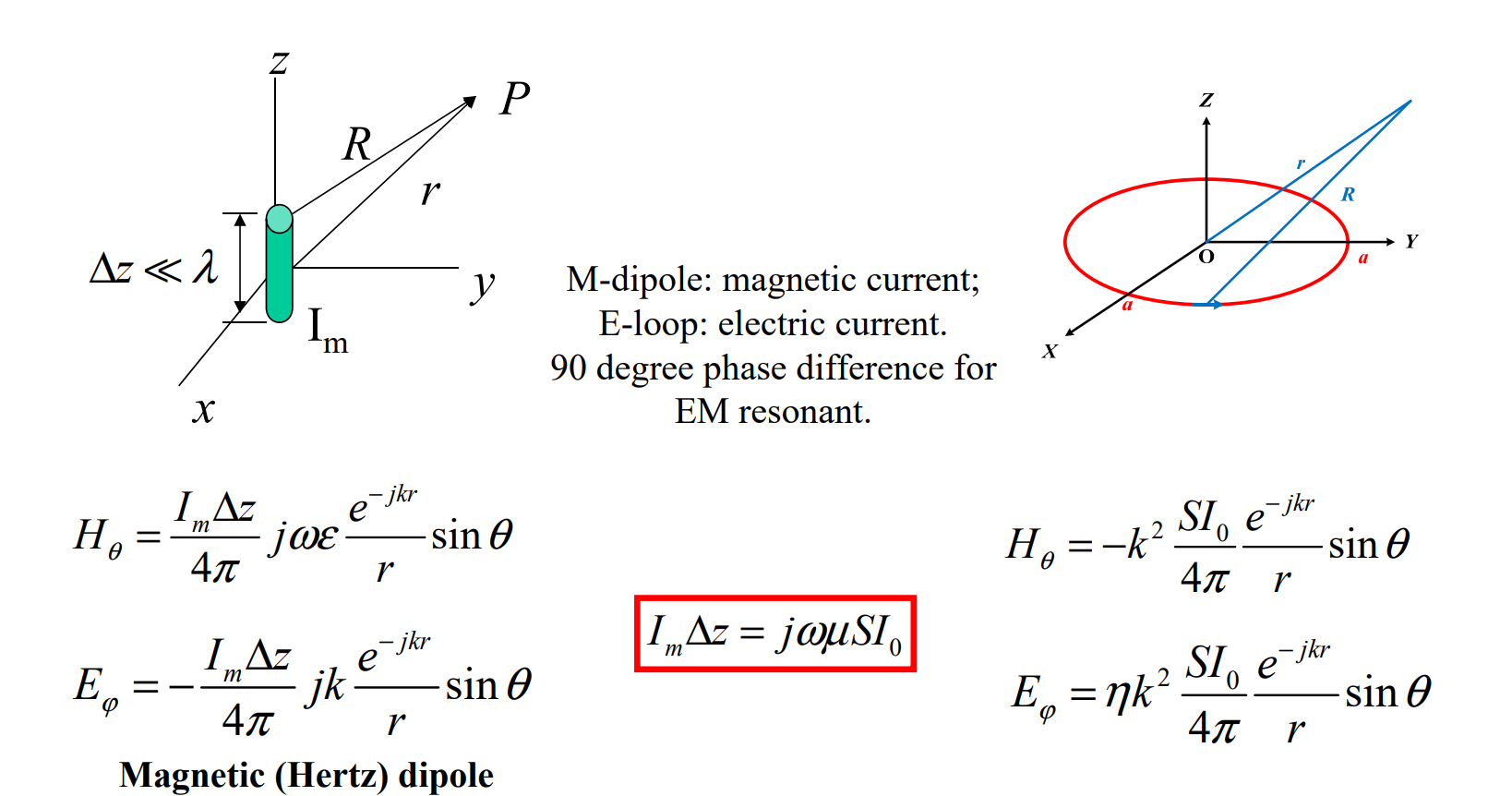
Loop Antennas

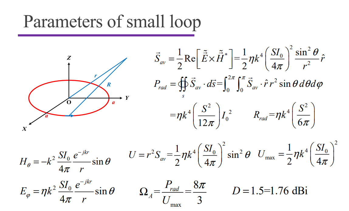
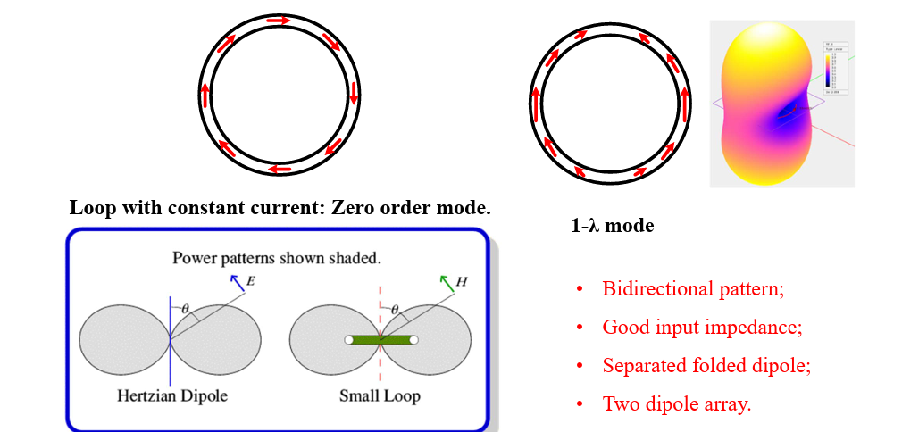
Small Loop

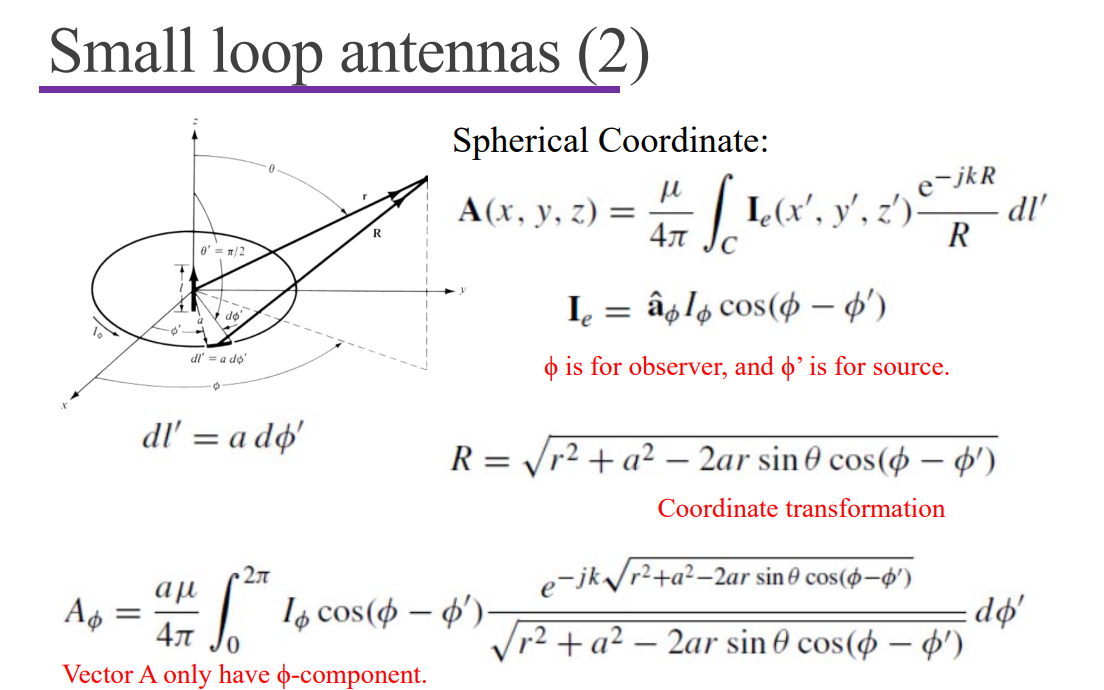
Infinite small loop radius;

Infinite small wire radius;

Uniform distribution.

Resistance $R_r$ too small!

Finite-length loop antennas

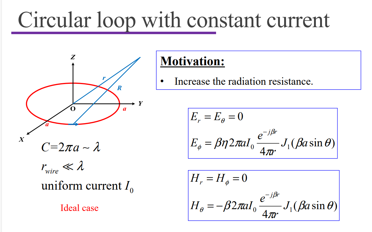
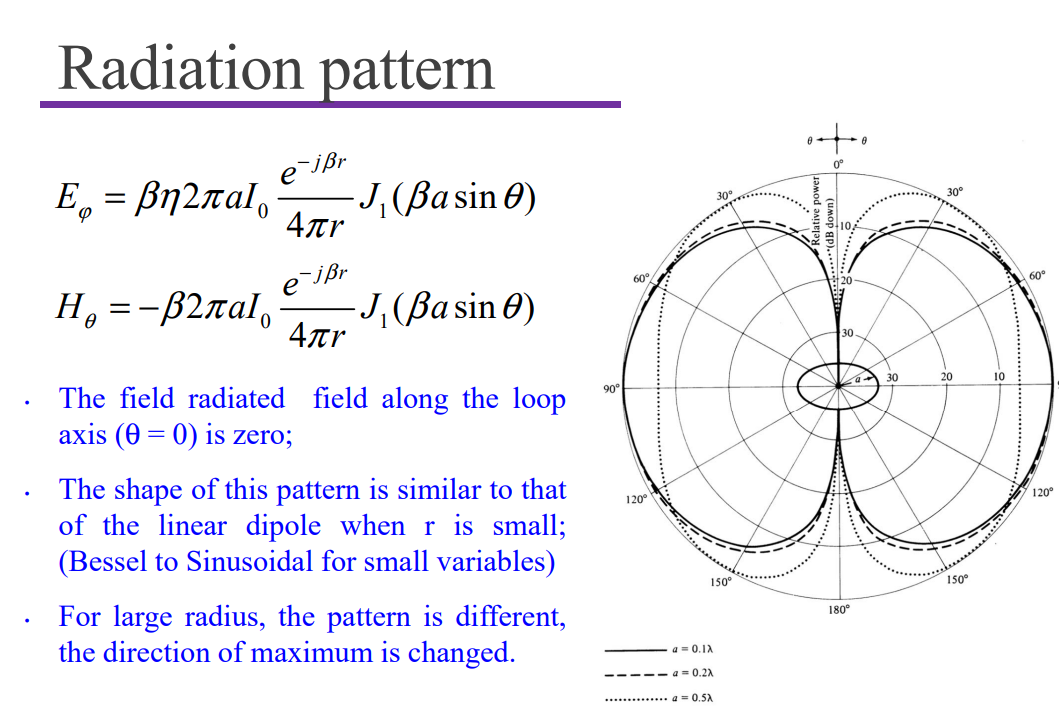
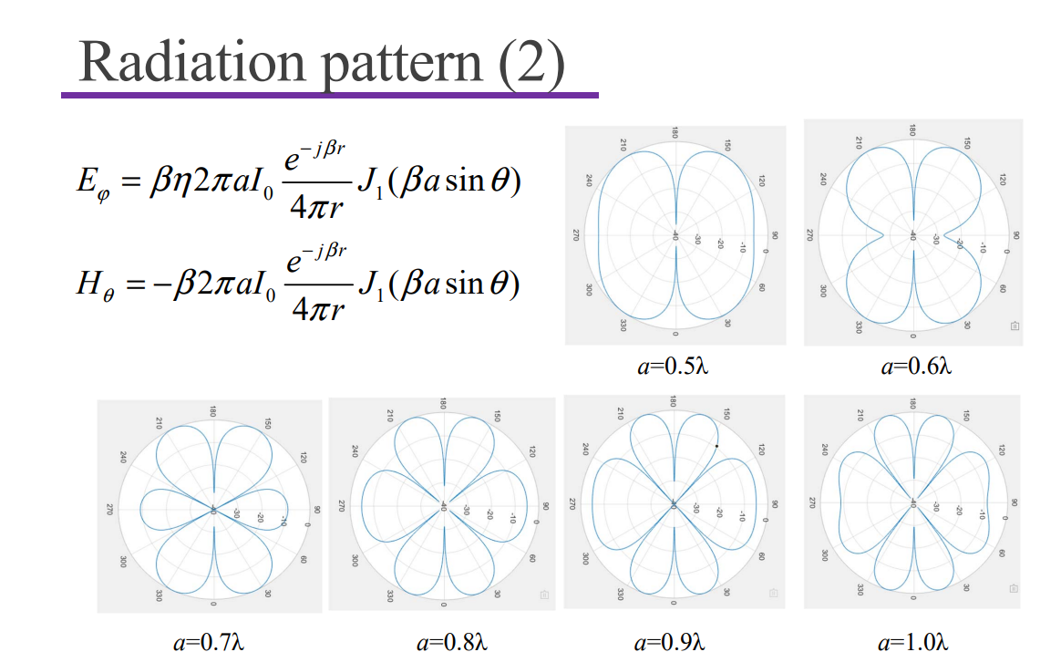
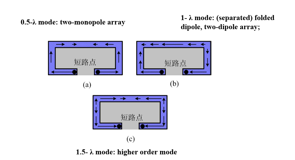
Modes of Loop antennas

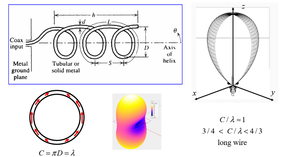
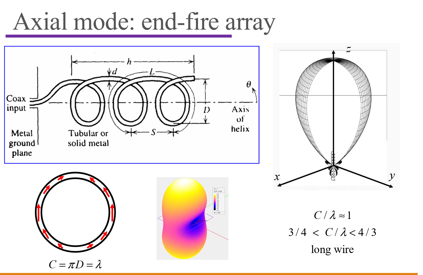
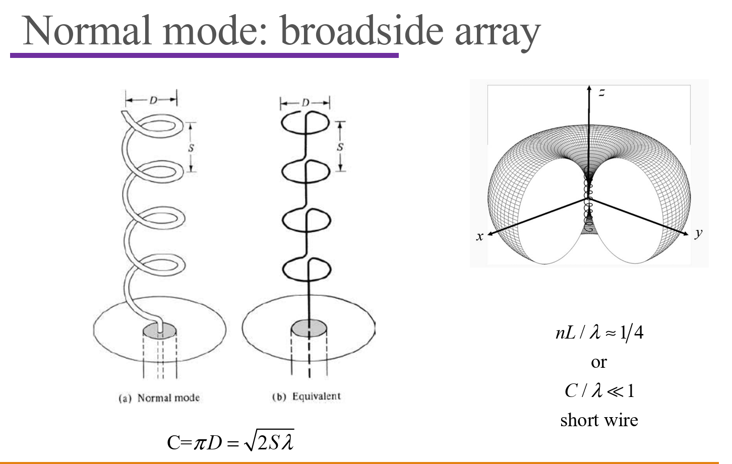
Helix/helical antennas

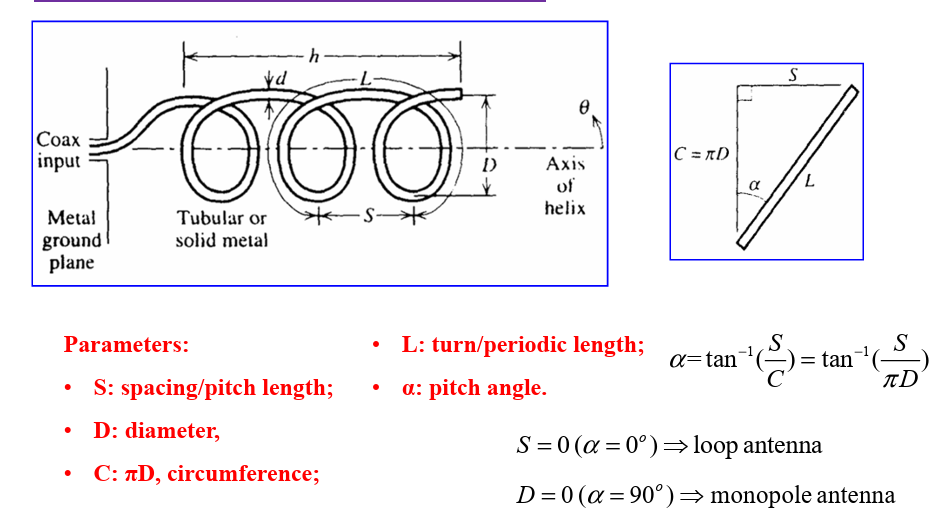
Axial Mode

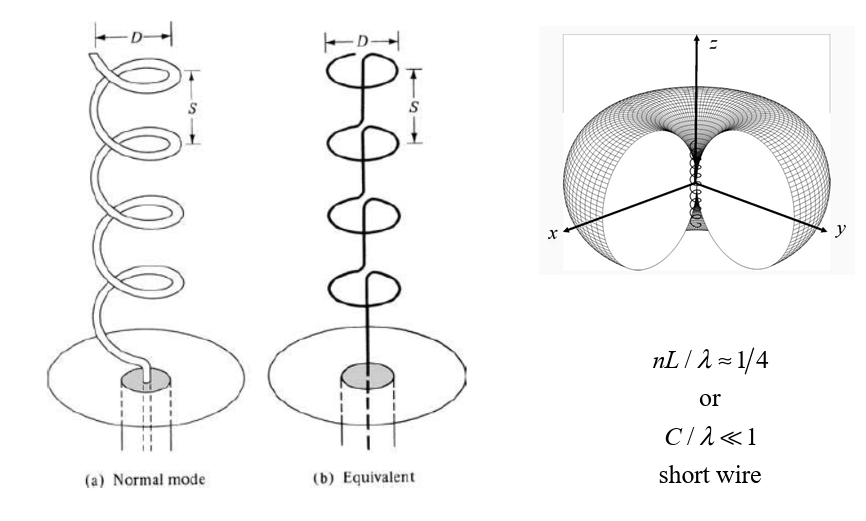
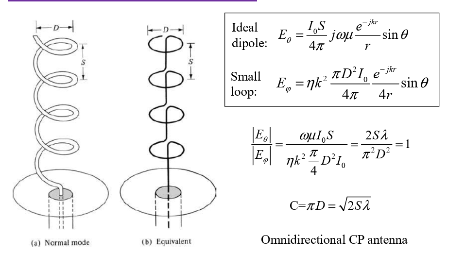
Normal Mode:

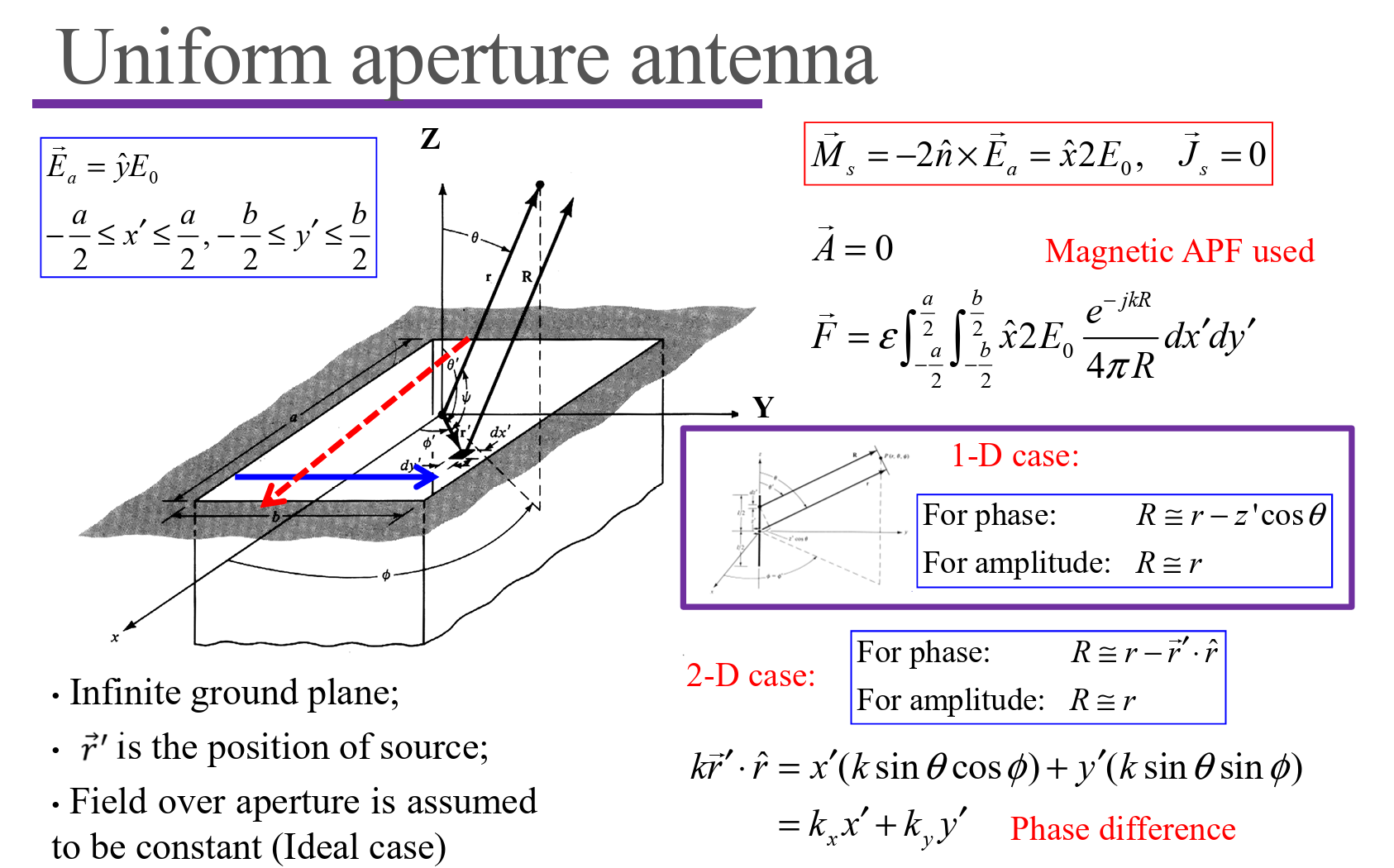
Aperture Antenna

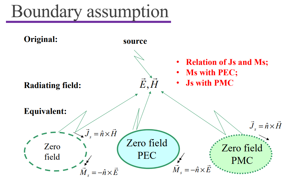
Huygens’ Principle

Rectangular aperture antennas

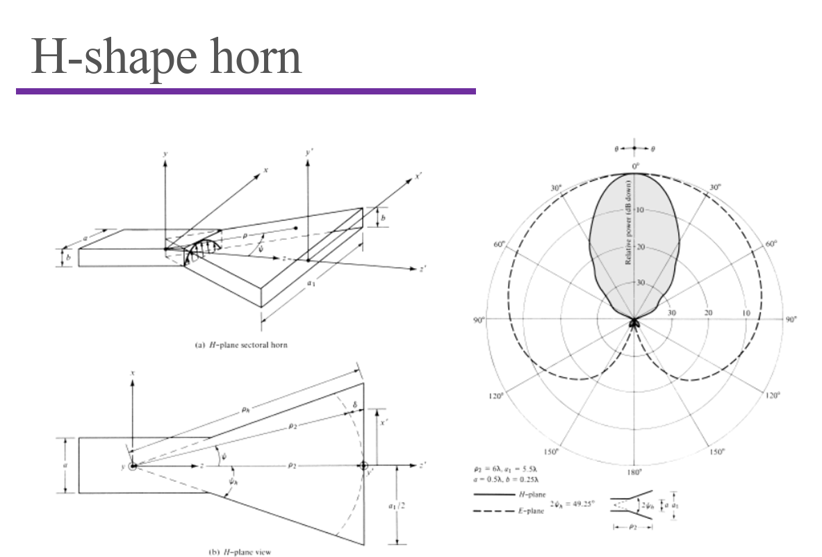
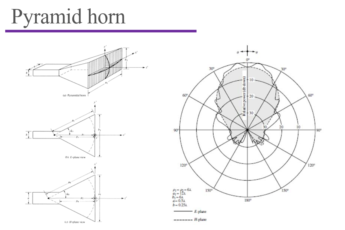
Horn Antennas

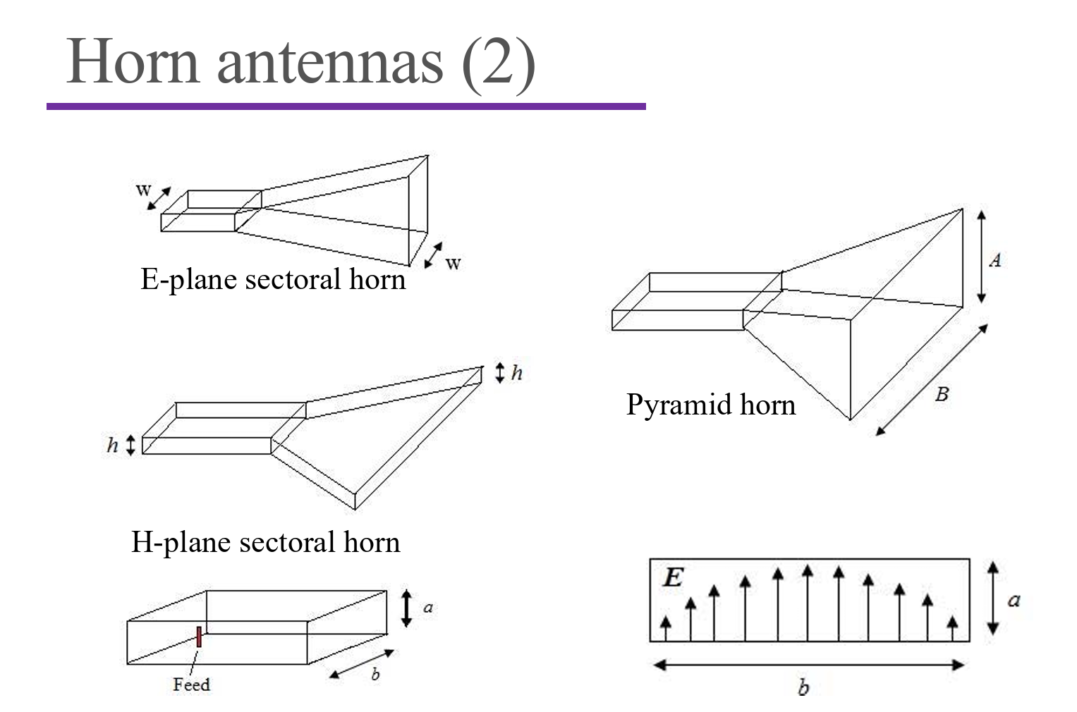
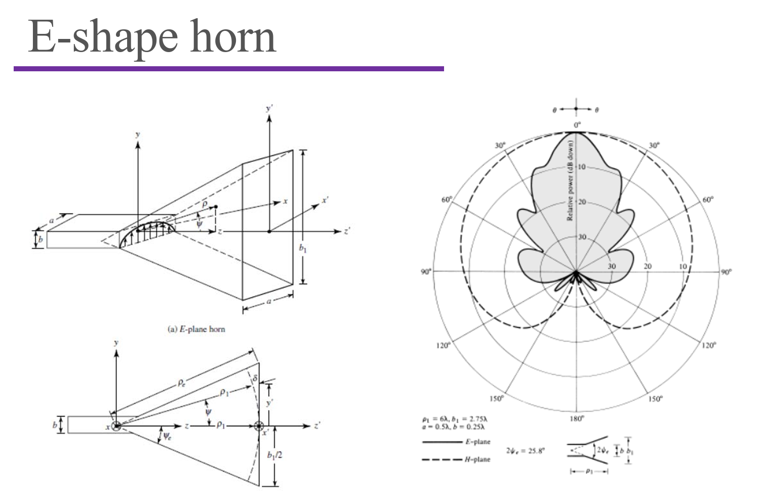
The E-pattern is in shadow.

Antenna Array

1-D Linear Array

2-D Planar Array

3-D Conformal Array

Array Element

• Dipoles
• Loops
• Slots
• Microstrip antennas

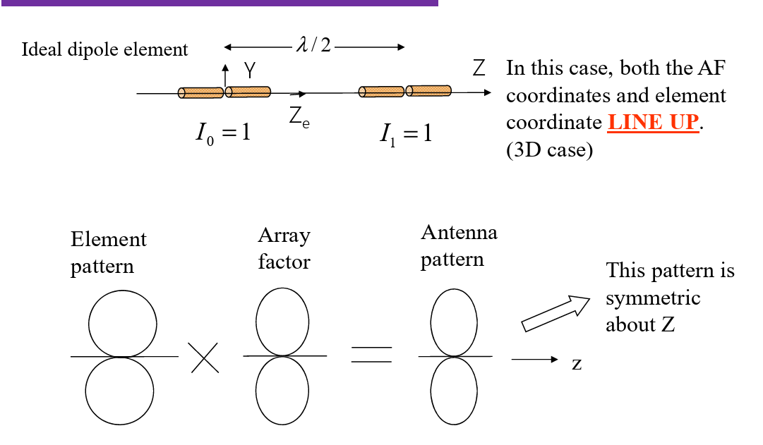
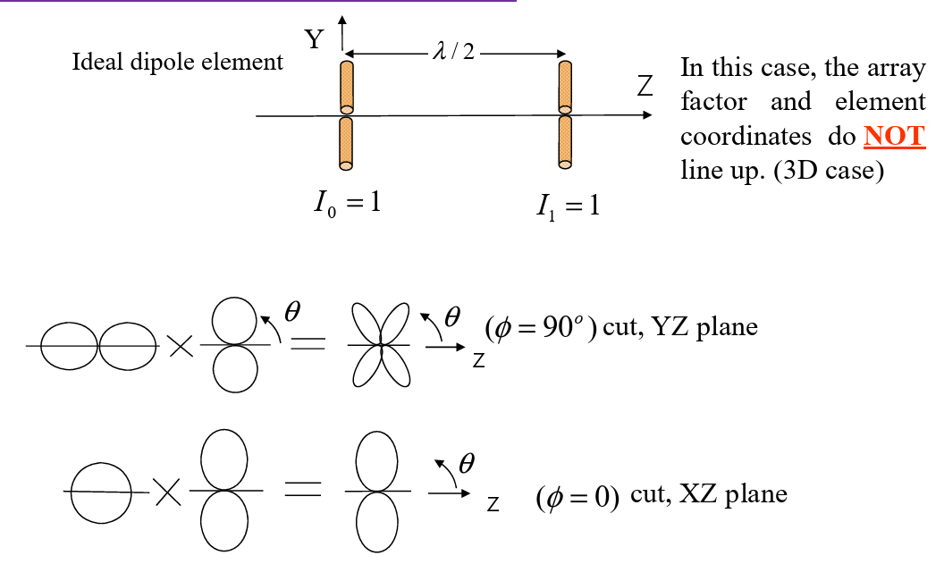
Two-Element array

$$ \begin{gathered} \vec{E}_1= \hat{\theta}\frac{I\Delta z}{4\pi}j\omega\mu\frac{e^{-jkr_1}}{r_1}\cos\theta_1 \\ \vec{E}_{2}= \hat{\theta}\frac{I\Delta z}{4\pi}j\omega\mu\frac{e^{-jkr_2}}{r_2}\cos\theta_2 \end{gathered} $$

Remarks:

• Two element;
• Towards Y axis;
• Along Z axis;
• Space: d;
• Uniform phase
  and amplitude;
• Observe in 2D
  (YZ-plane).

Far field Approximation

$$ \begin{aligned}&\vec{E}_{total}=\vec{E}_1+\vec{E}_2\\&=\hat{\theta}\frac{I\Delta z}{4\pi}j\omega\mu\cos\theta\frac1r\Bigg(e^{-jk(r-\frac d2\cos\theta)}+e^{-jk(r+\frac d2\cos\theta)}\Bigg)\end{aligned} $$ $$ \begin{aligned} \vec{E}_{total}& =\vec{E}_1+\vec{E}_2=\hat{\theta}\frac{I\Delta z}{4\pi}j\omega\mu\cos\theta\frac{1}{r}\Bigg(e^{-jk(r-\frac{d}{2}\cos\theta)}+e^{-jk(r+\frac{d}{2}\cos\theta)}\Bigg) \\ &=\hat{\theta}\frac{I\Delta z}{4\pi}j\omega\mu\cos\theta\frac{e^{-jkr}}{r}\Bigg(e^{jk\frac{d}{2}\cos\theta}+e^{-jk\frac{d}{2}\cos\theta}\Bigg) \\ &=\hat{\theta}\underbrace{\frac{I\Delta z}{4\pi}j\omega\mu\cos\theta\frac{e^{-jkr}}r}_{\text{Element pattern}}\underbrace{2\cos\biggl[\frac12kd\cos\theta\biggr]}_{\text{Array Factor (AF)}} \end{aligned} $$

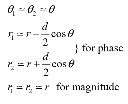
Remarks:

• Uniform phase and amplitude;
• AF is related to space (d);
• AF is with no relation with antenna type.

$$ AF{=}2\cos\left[\frac12kd\cos\theta\right]\quad kd{=}\frac{2\pi}\lambda d{=}2\pi\frac d\lambda $$

N-Element array

$$ \begin{aligned}&AF=1+e^{jkd\cos\theta}+e^{j2kd\cos\theta}+\cdots+e^{j(N-1)kd\cos\theta}\\&=\sum_{n=1}^Ne^{j(n-1)kd\cos\theta}=\sum_{n=1}^Ne^{j(n-1)\Psi}\end{aligned} $$ $$ AF=1+e^{j\Psi}+e^{j2\Psi}+\cdots+e^{j(N-1)\Psi}=\frac{e^{jN\Psi}-1}{e^{j\Psi}-1}\\=\frac{e^{j\frac N2\Psi}\left(e^{j\frac N2\Psi}-e^{-j\frac N2\Psi}\right)}{e^{j\frac12\Psi}\left(e^{j\frac12\Psi}-e^{-j\frac12\Psi}\right)}=\frac{e^{j\frac N2\Psi}\sin\left(\frac N2\Psi\right)}{e^{j\frac12\Psi}\sin\left(\frac12\Psi\right)} $$

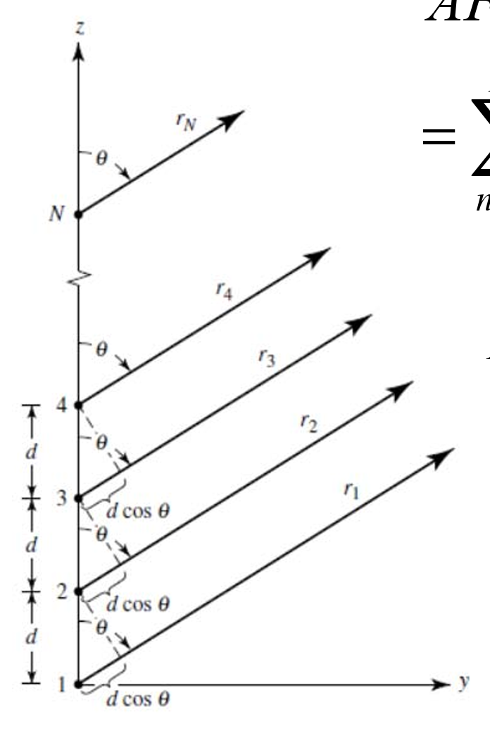
Refenece Point at the end:

$$ AF=\frac{e^{j\frac N2\Psi}\sin\left(\frac N2\Psi\right)}{e^{j\frac12\Psi}\sin\left(\frac12\Psi\right)},\Psi=kd\cos\theta, $$

Refenece Point at the center:

$$ AF=\frac{\sin\left(\frac N2\Psi\right)}{\sin\left(\frac12\Psi\right)},\Psi=kd\cos\theta, $$

In Progreessive Phase Shift:

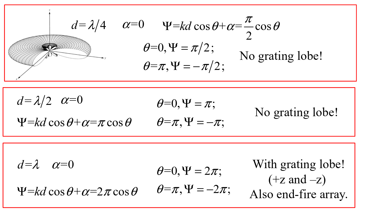
$$ \Psi=kd\cos\theta+\alpha $$ $$ AF=1+e^{j(kd\cos\theta+\alpha)}+e^{j2(kd\cos\theta+\alpha)}+\cdots+e^{j(N-1)(kd\cos\theta+\alpha)}\\=\sum_{n=1}^Ne^{j(n-1)(kd\cos\theta+\alpha)}=\sum_{n=1}^Ne^{j(n-1)\Psi}=\frac{e^{j\frac N2\Psi}\sin\left(\frac N2\Psi\right)}{e^{j\frac12\Psi}\sin\left(\frac12\Psi\right)} $$

Normalized Array Factor:

$$ \left|f(\Psi)\right|=\left|\frac{\sin\left(\frac N2\Psi\right)}{N\sin\left(\frac12\Psi\right)}\right| $$

Grating Lobe:

$$ \begin{aligned} \theta\in\begin{bmatrix}0,\pi\end{bmatrix}\text{ or }\theta\in\begin{bmatrix}\theta_1,\theta_2\end{bmatrix}\text{, visible region} \\ \text{In the visible region,} \\ ifwehaveY= 0\mathrm{~and~}\Psi=2\pi. \end{aligned} $$

Avoid grating lobe:

1. Smaller d;
2. Smaller phase shift.

$$ 1.\mathrm{~For~}\alpha=\pi\Rightarrow2kd<2\pi\Rightarrow d\mathrm{~/~}\lambda<\frac12\\2.\mathrm{~For~}\alpha=0\mathrm{~}\Rightarrow\mathrm{~k}d<2\pi\Rightarrow d\mathrm{~/~}\lambda<1 $$

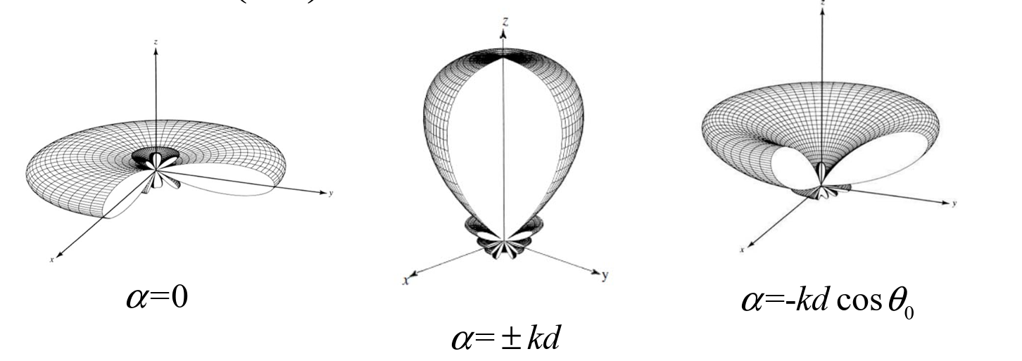
Broadside Array

Maximum @ $\theta = 90\degree$

$$ AF\boldsymbol{=}N@\boldsymbol{\theta}\boldsymbol{=}\boldsymbol{\pi}/2\quad\boldsymbol{\Psi}\boldsymbol{=}kd\cos\boldsymbol{\theta}\boldsymbol{+}\boldsymbol{\alpha}|_{\theta=\pi/2}\boldsymbol{=}0 $$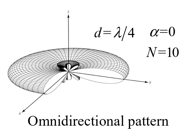

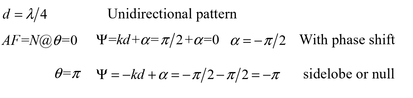
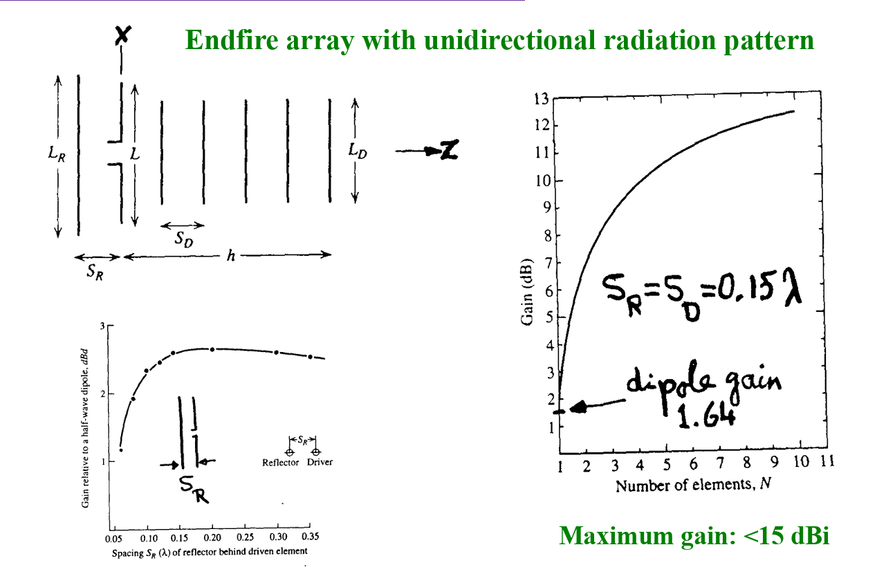
End-fire Array

$$ \begin{aligned} &AF= N@\theta{=}0 &\Psi=kd+\alpha=2n\pi(n=0,\pm1,\pm2\ldots) \\ &\text{or} \\ &AF= N@\theta{=}\pi &\Psi=-kd+\alpha=2n\pi(n=0,\pm1,\pm2...) \\ &\Psi=kd\cos\theta+\alpha=2\pi\cos\theta \end{aligned} $$

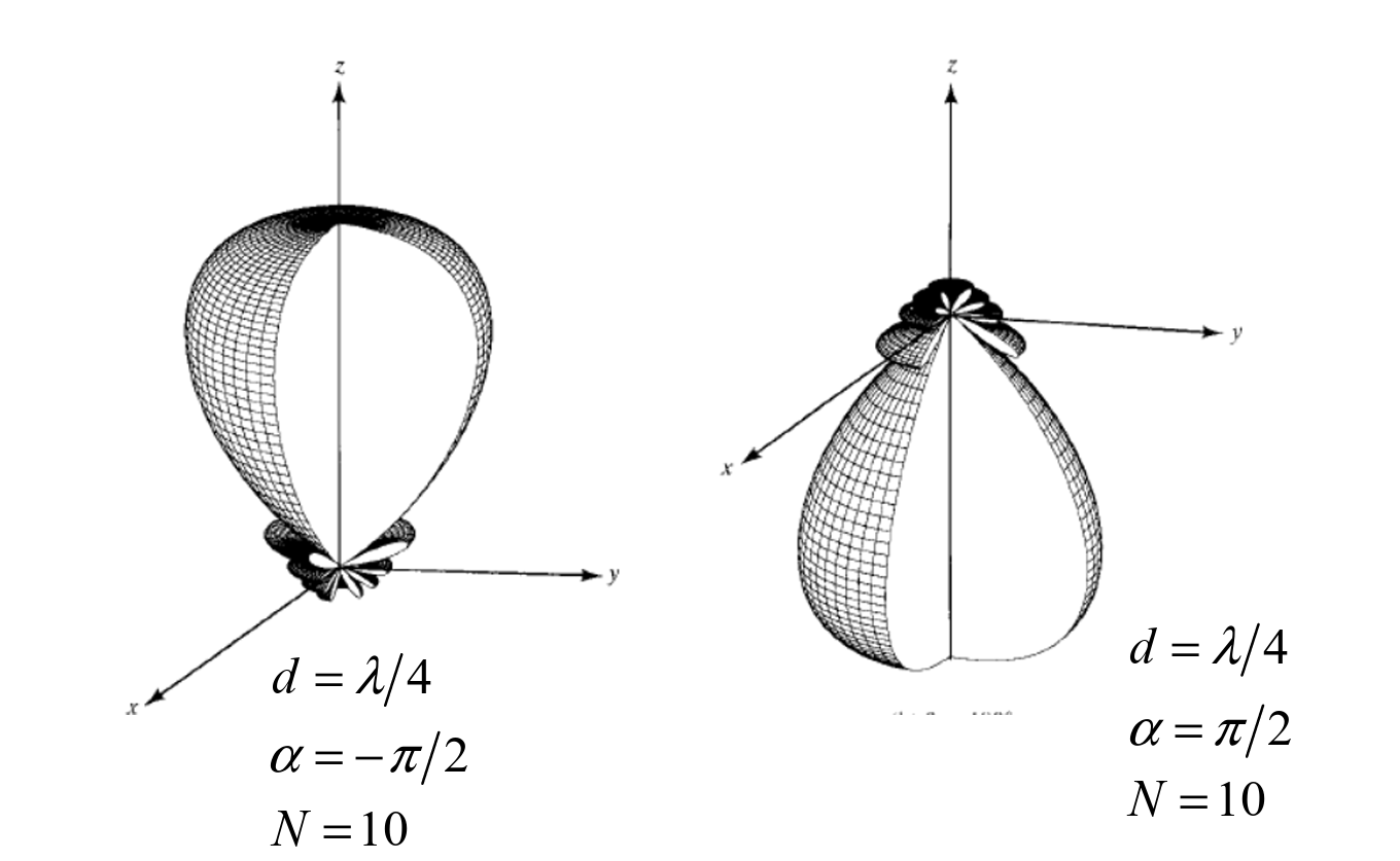
Bidirectional:

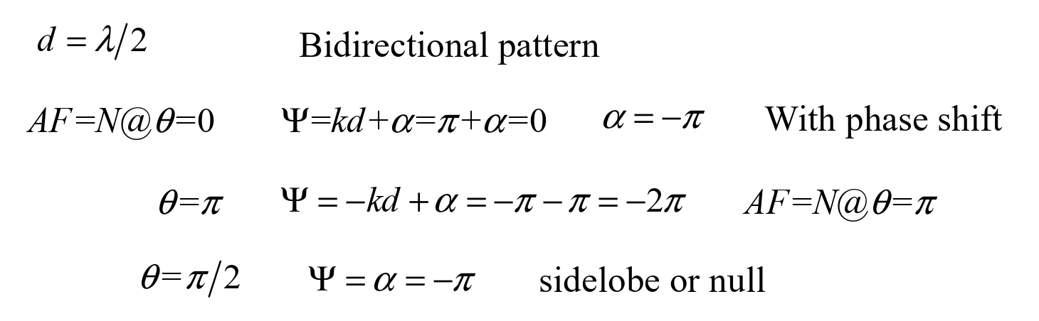
Unidirectional:

Phased Array

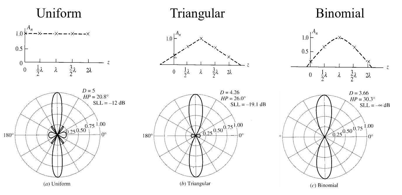
Non-uniform Array

Side Lobe

Uniform array:

• Universal pattern: N↑, SLL↓
• With a limit of -13.3 dB
• No control of SL

How to reduce SLL?

Non-uniform excitation

Planar Array

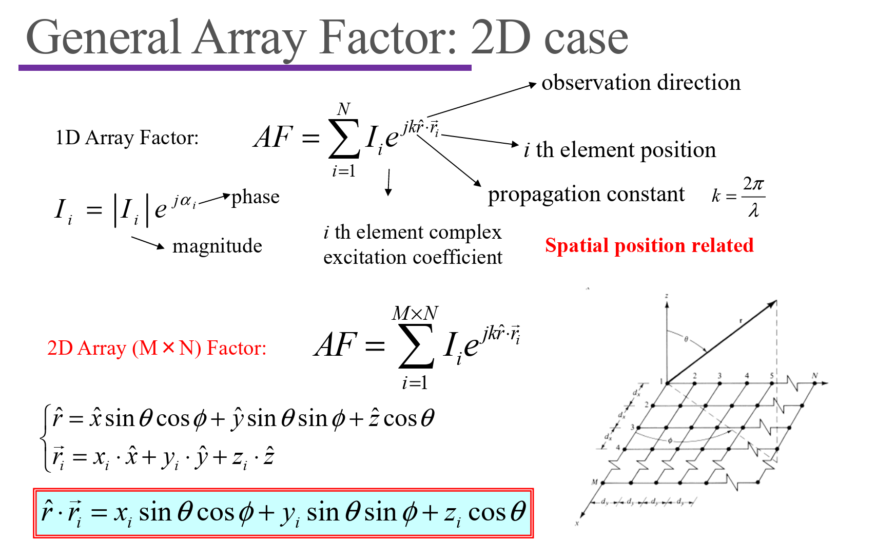
Can be viewed as product of two linear array factors:

$$ AF=\sum_{i=1}^{M\times N}I_ie^{jk\hat{r}\cdot\vec{r}_i}\\ AF_n(\theta,\phi)=\left\{\frac{\sin(\frac M2\psi_x)}{M\sin\frac{\psi_x}2}\right\}\left\{\frac{\sin(\frac N2\psi_y)}{N\sin\frac{\psi_y}2}\right\};\\\psi_x=kd_x\sin\theta\cos\varphi+\alpha_x\\\psi_y=kd_y\sin\theta\sin\varphi+\alpha_y $$

Applications

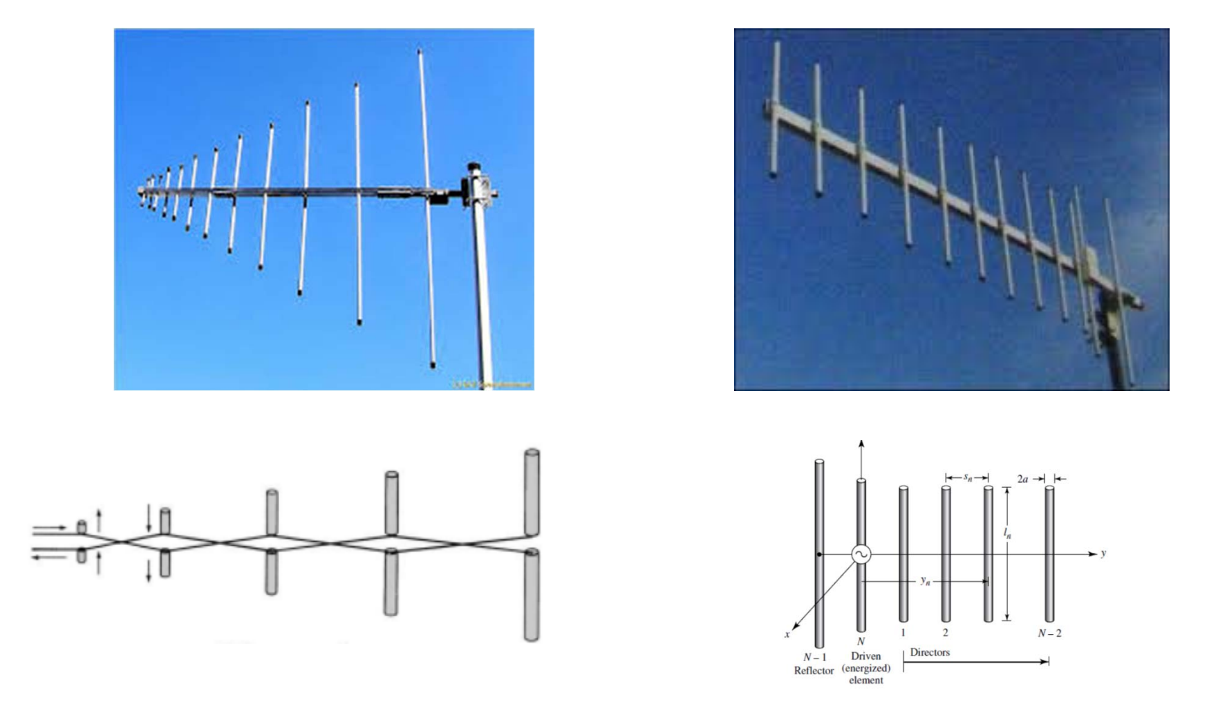
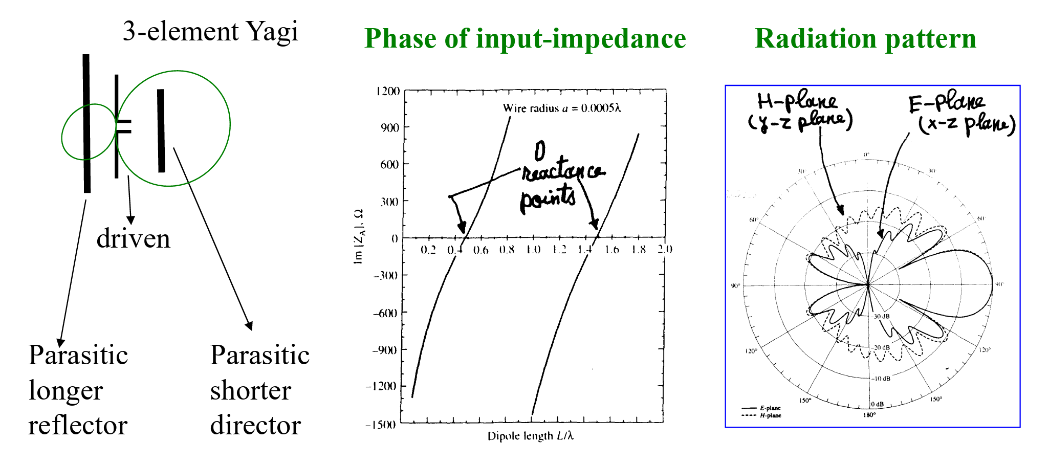
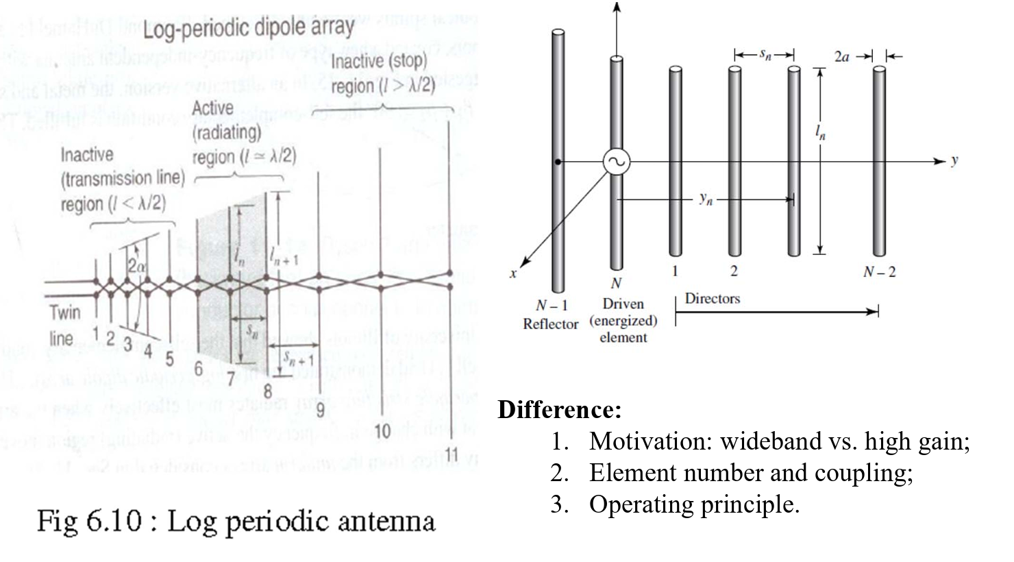
Yagi-Uda Antenna

Basic configuration:

• One driven element;
• Two parasitic elements or more

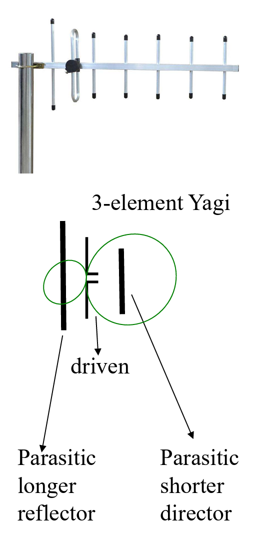
Remarks:

• Parasitic elements are excited by near-field coupling from the driven element;
• Proper design of parasitic elements for end fire radiation;
• In far field, the radiated waves from all the elements are in-phase.

Helix Antenna

Travelling-Wave Antennas

Travelling wave & standing wave

Long wire antennas

Note:
Long wire antennas: “l” = Several wavelength

• One end for excitation;
• The other end for load (open, short, or matching);
• Transmission line with radiation.

Log-periodic Antennas

Yagi-Uda: High Gain

Log-periodic: Wide Bandwidth

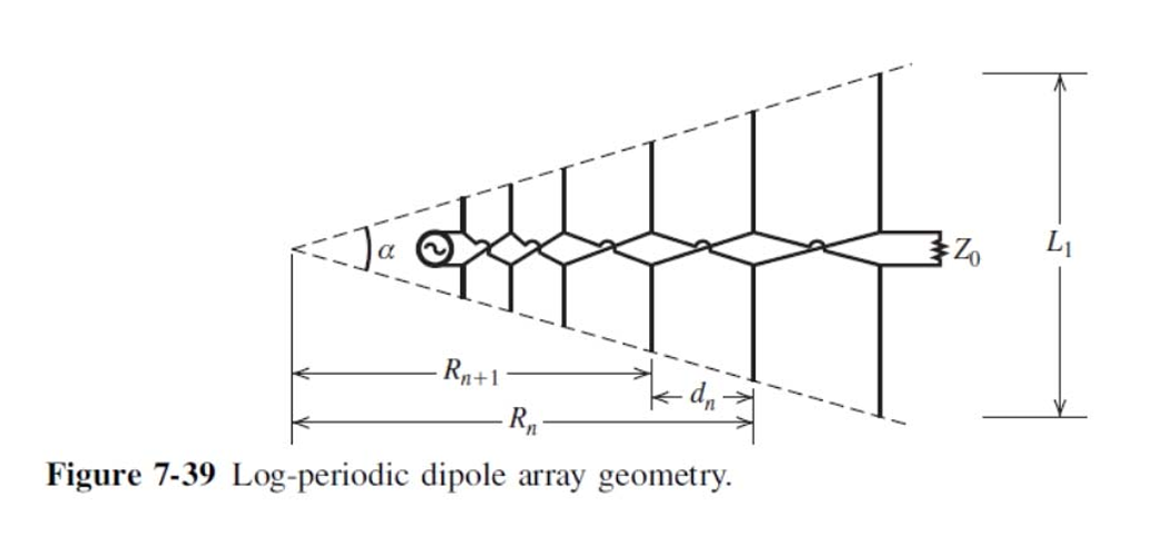
Why:

1. Feed from smaller dipole element;
2. Feed out-of-phase with adjacent elements;
3. Add a resistor at the end.

$$ \tau=\frac{R_{n+1}}{R_{n}}=\frac{L_{n+1}}{L_{n}}=\frac{d_{n+1}}{d_{n}}\\\alpha=2\tan^{-1}\left(\frac{1-\tau}{4\sigma}\right)\\\sigma=\frac{d_{n}}{2L_{n}}\\L_{1}\approx\frac{\lambda_{L}}{2}\quad\mathrm{and}\quad L_{N}\approx\frac{\lambda_{U}}{2} $$

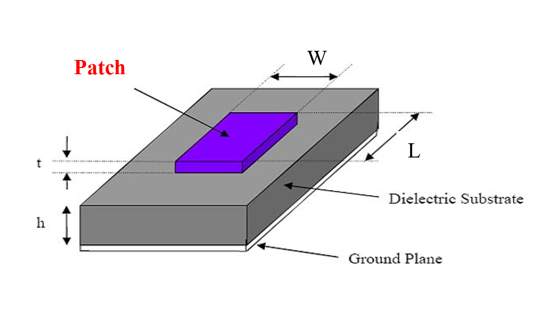
Microstrip Antennas

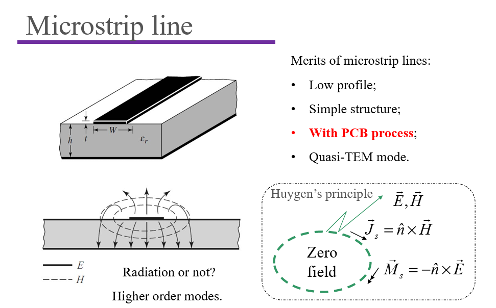
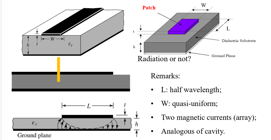
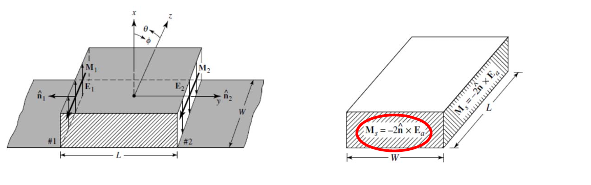
Basic Mode

• Equivalent magnetic current;
• Radiating and non-radiating apertures;
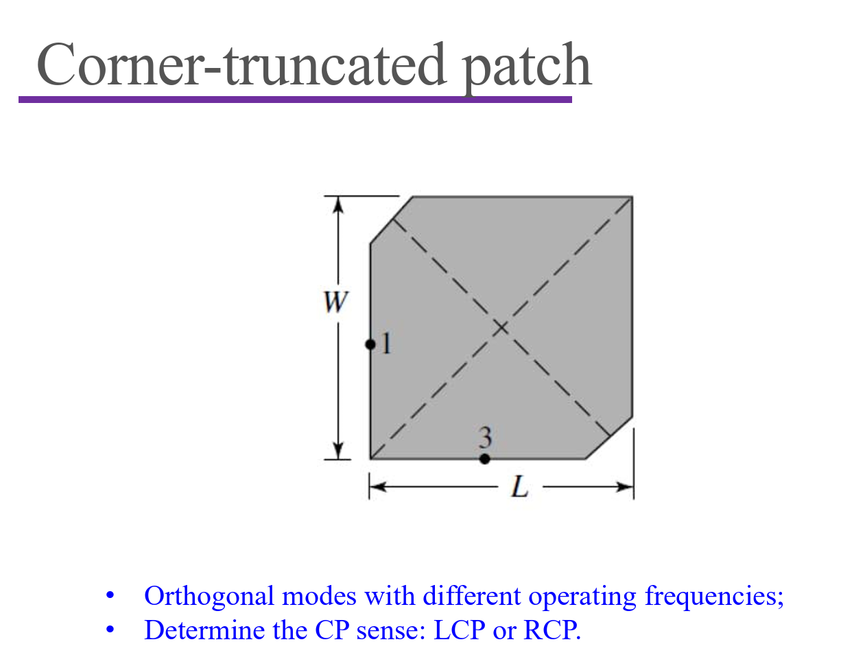
• Operating frequency with different L.

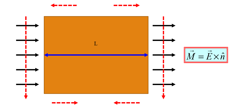
• Magnetic current array;
• Image theorem from infinite ground;
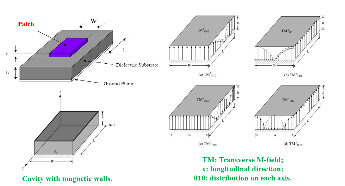
• Cavity model with magnetic walls;
• Different from

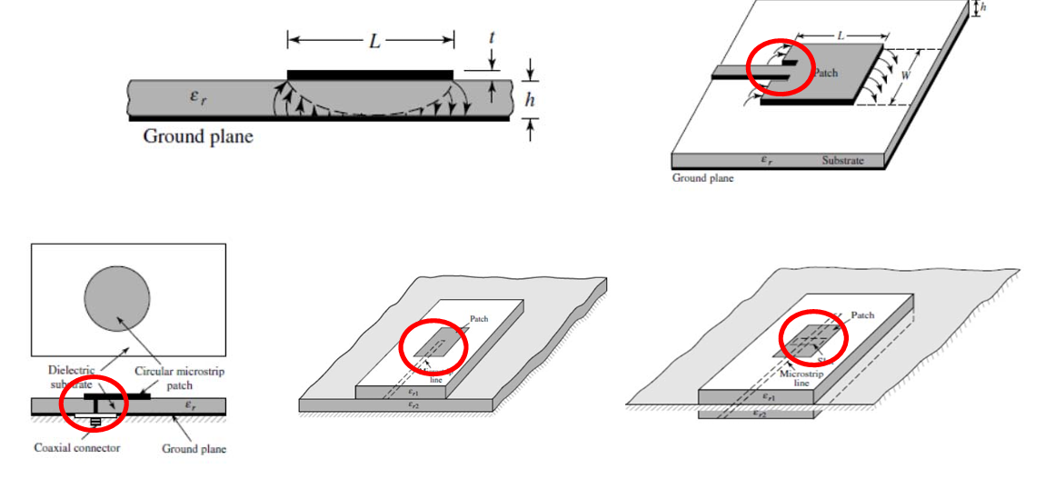
Antenna feeding methods

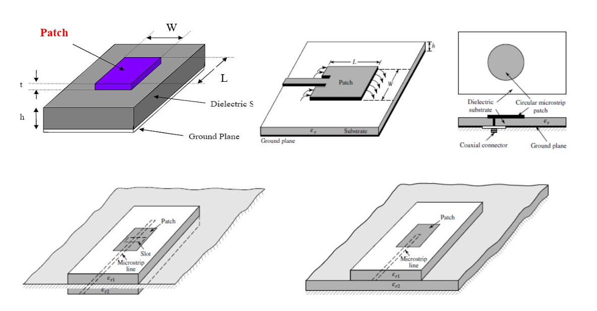
Impedance Matching:

Using 50-Ohm port: finding the position with Z_in=50 Ohm

Analysis Model

Known:

• Operating Frequency
• Dielectric: $\varepsilon_r$ and $h$
• Metal: $t$

Design:

• Patch: $L$ and $W$
• Evaluate gain

2 Models:

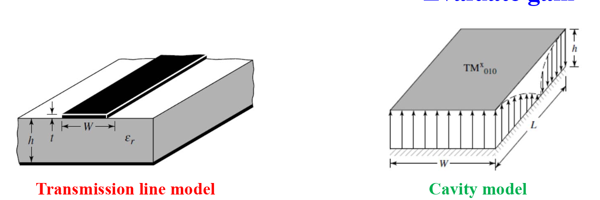
Transmission line model

determine W

Uniform distribution and field intensity in dielectric

$$ W=\frac{1}{2f_r\sqrt{\mu_0\epsilon_0}}\sqrt{\frac{2}{\epsilon_r+1}} $$

Effective permittivity

$$ \varepsilon_{eff}=\frac{\varepsilon_r+1}2+\frac{\varepsilon_r-1}2{\left[1+12\frac hW\right]}^{-1/2} $$

Fring effect and determine L

$$ \frac{\Delta L}{h}=0.412\frac{(\varepsilon_{eff}+0.3)(\frac Wh+0.264)}{(\varepsilon_{eff}-0.258)(\frac Wh+0.8)}\\L=\frac{\lambda_d}2-2\Delta L=\frac{\lambda_0}{2\sqrt{\varepsilon_{eff}}}-2\Delta L $$

impedance matching

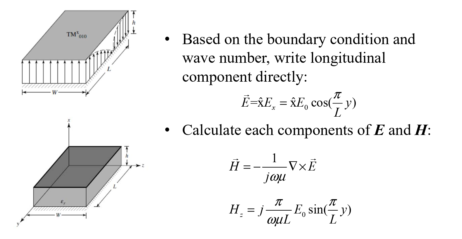
Cavity Model

Circular polarization

Dual feed patch

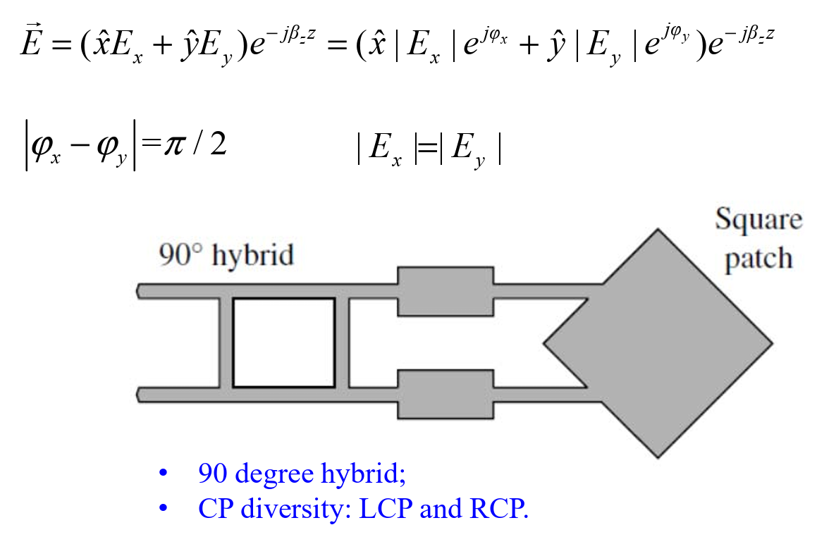
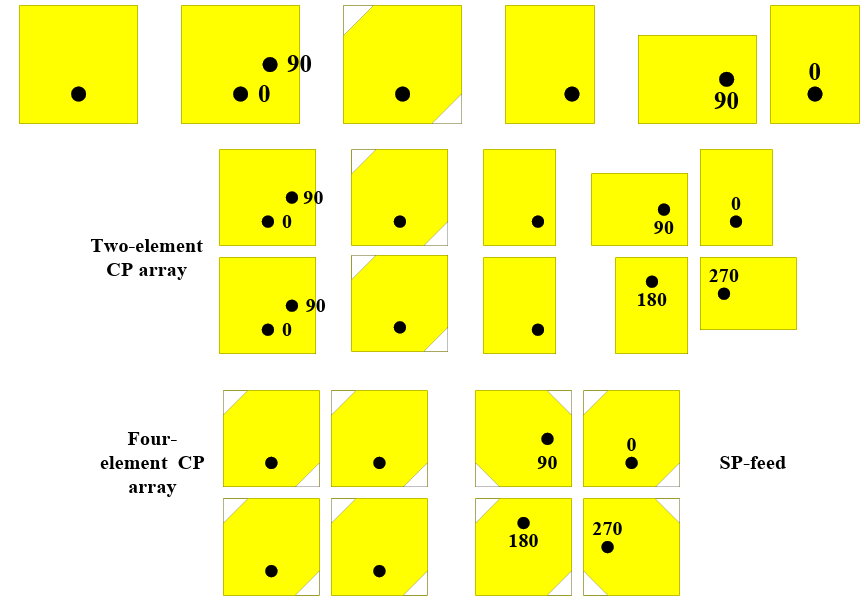
SP-feed 旋转馈电

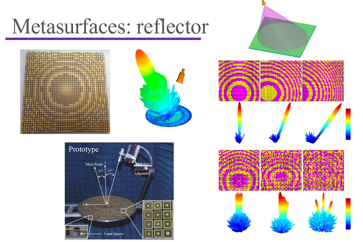
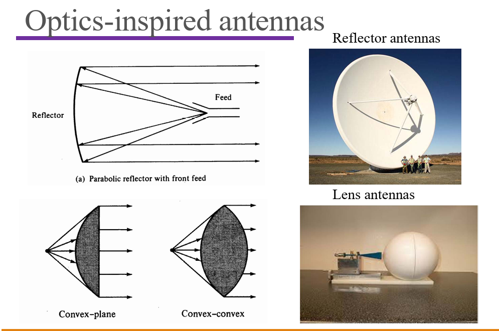
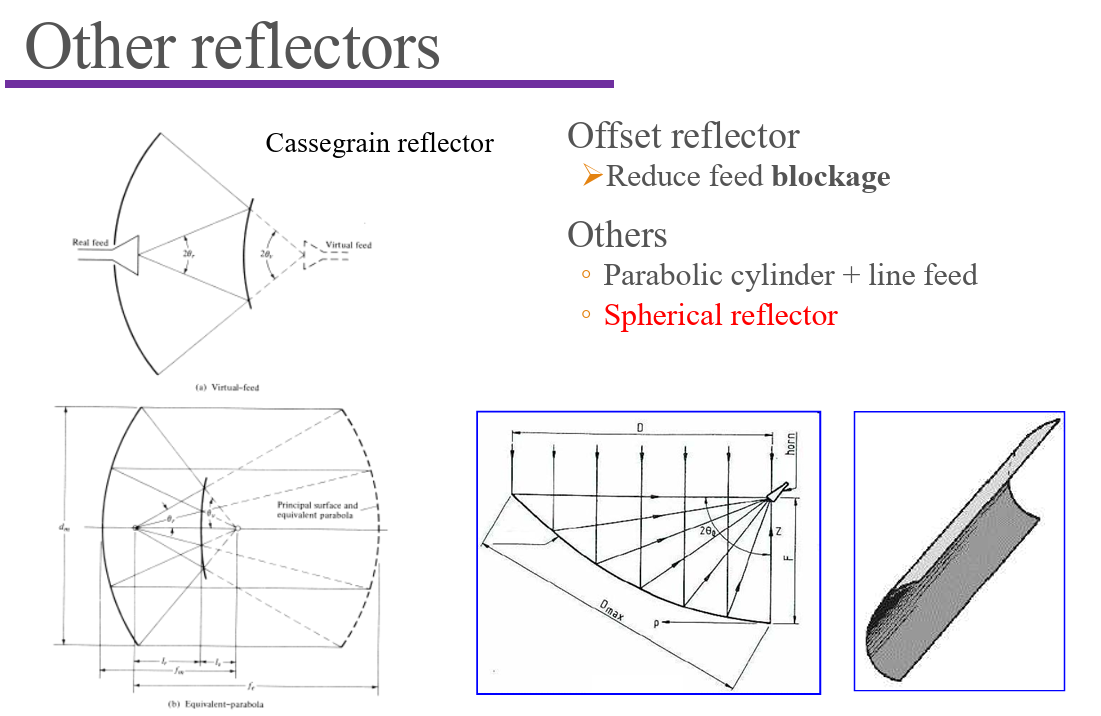
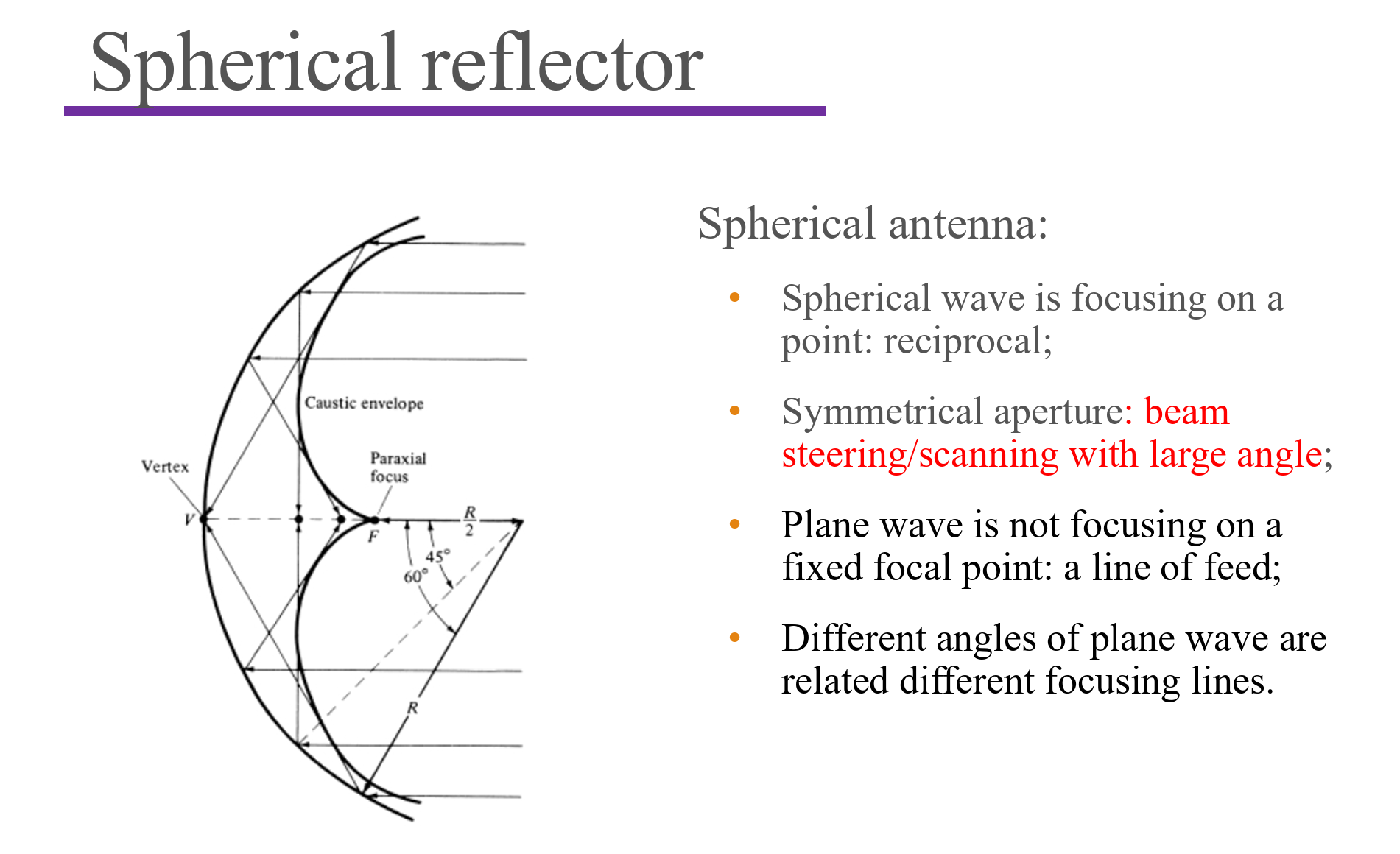
Reflector and lens antennas

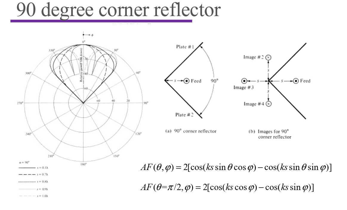
Corner Reflectors

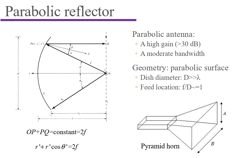
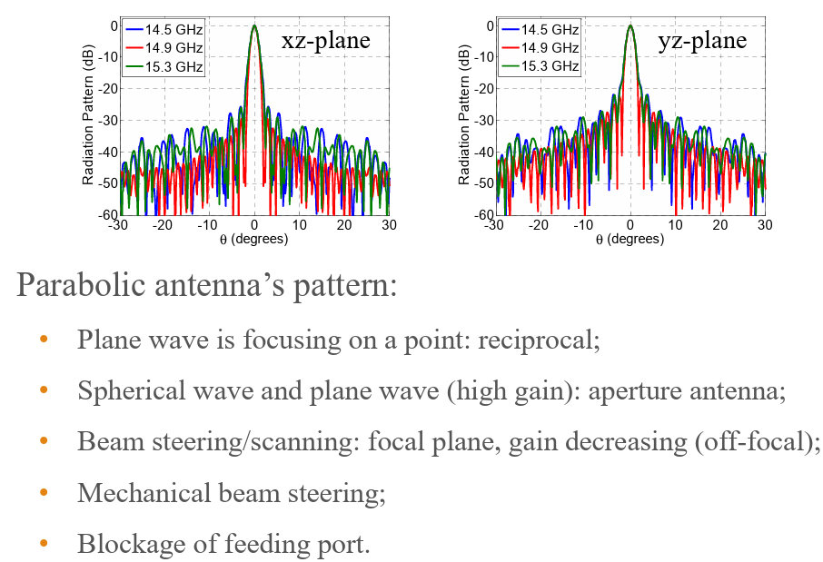
Parabolic Reflectors

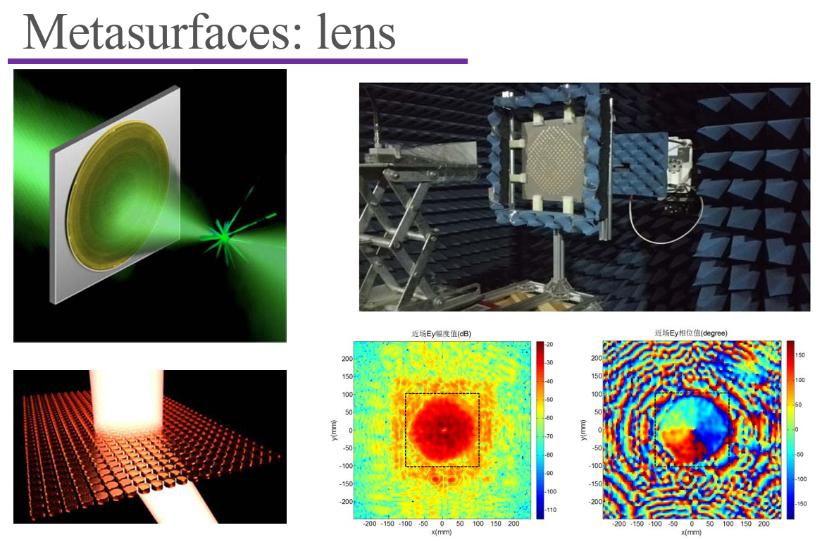
Lens Antennas

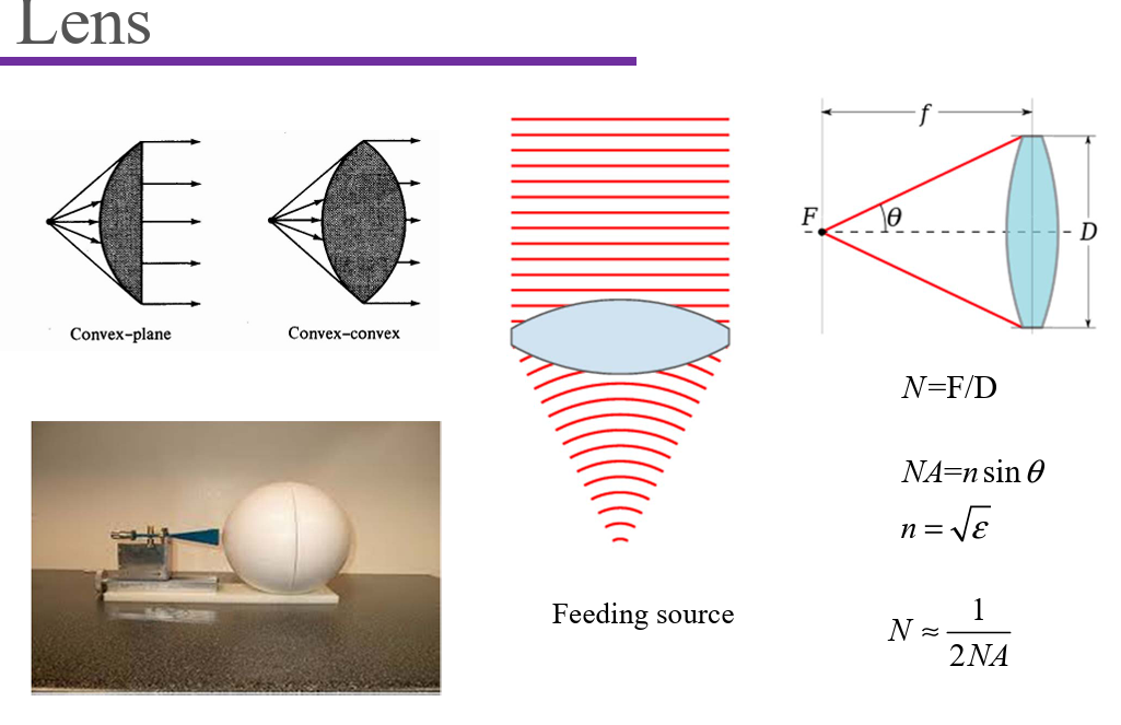
Lens antennas:

• High gain: plane wave;
• Geometrical optics: equal optical distance;
• Source: spherical wave, illuminate the whole lens;
• Source is positioned on the focal point for normal
  radiated plane wave;
• Other incident/radiated angle of plane wave: focus on
  the focal plane with gain decrease;
• Spatial Fournier Transformation: (x, y)&k

Reflected and transmitted array